| Type: | Package |
| Version: | 5.0 |
| Date: | 2025-12-14 |
| Title: | Simulation of Diffusion Processes |
| Author: | Arsalane Chouaib Guidoum
 [cre, aut],
Kamal Boukhetala [aut] [cre, aut],
Kamal Boukhetala [aut] |
| Maintainer: | Arsalane Chouaib Guidoum <acguidoum@univ-tam.dz> |
| Depends: | R (≥ 4.0.0) |
| Imports: | Deriv (≥ 3.8.0), MASS (≥ 7.3-30), parallel |
| Suggests: | deSolve (≥ 1.11), knitr (≥ 1.10), rgl (≥ 0.93.991), rmarkdown (≥ 0.8), scatterplot3d (≥ 0.3-36), sm (≥ 2.2-5.3) |
| BugReports: | https://github.com/acguidoum/Sim.DiffProc/issues |
| URL: | https://github.com/acguidoum/Sim.DiffProc |
| VignetteBuilder: | knitr |
| Encoding: | UTF-8 |
| Description: | It provides users with a wide range of tools to simulate, estimate, analyze, and visualize the dynamics of stochastic differential systems in both forms Ito and Stratonovich. Statistical analysis with parallel Monte Carlo and moment equations methods of SDEs <doi:10.18637/jss.v096.i02>. Enabled many searchers in different domains to use these equations to modeling practical problems in financial and actuarial modeling and other areas of application, e.g., modeling and simulate of first passage time problem in shallow water using the attractive center (Boukhetala K, 1996) ISBN:1-56252-342-2. |
| License: | GPL-2 | GPL-3 [expanded from: GPL (≥ 2)] |
| Classification/MSC: | 37H10, 37M10, 60H05, 60H10, 60H35, 60J60, 65C05, 68N15, 68Q10 |
| RoxygenNote: | 7.3.3 |
| NeedsCompilation: | no |
| Packaged: | 2025-12-13 15:59:28 UTC; stars |
| Repository: | CRAN |
| Date/Publication: | 2025-12-13 17:00:08 UTC |
Simulation of Diffusion Processes
Description
It provides users with a wide range of tools to simulate, estimate, analyze, and visualize the dynamics of stochastic differential systems in both forms Ito and Stratonovich. Statistical analysis with parallel Monte Carlo and moment equations methods of SDEs <doi:10.18637/jss.v096.i02>. Enabled many searchers in different domains to use these equations to modeling practical problems in financial and actuarial modeling and other areas of application, e.g., modeling and simulate of first passage time problem in shallow water using the attractive center (Boukhetala K, 1996) ISBN:1-56252-342-2.
Details
| Package: | Sim.DiffProc |
| Type: | Package |
| Version: | 5.0 |
| Date: | 2025-12-14 |
| License: | GPL (>= 2) |
| Depends: | R (>= 4.0.0) |
| Imports: | Deriv (>= 3.8.0), MASS (>= 7.3-30), parallel |
| Suggests: | deSolve (>= 1.11), knitr (>= 1.10), rgl (>= 0.93.991), rmarkdown (>= 0.8), scatterplot3d (>= 0.3-36), sm (>= 2.2-5.3) |
| Classification/MSC: | 37H10, 37M10, 60H05, 60H10, 60H35, 60J60, 65C05, 68N15, 68Q10 |
There are main types of functions in this package:
Simulation of solution to 1,2 and 3-dim stochastic differential equations of Itô and Stratonovich types, with different methods.
Simulation of solution to 1,2 and 3-dim diffusion bridge of Itô and Stratonovich types, with different methods.
Simulation the first-passage-time (f.p.t) in 1,2 and 3-dim sde of Itô and Stratonovich types.
Calculate symbolic ODE's of moment equations (means and variances-covariance) for 1,2 and 3-dim SDE's.
Monte-Carlo replicates of a statistic applied to 1,2 and 3-dim SDE's at any time t.
Computing the basic statistics (mean, var, median, ...) of the processes at any time t using the Monte Carlo method.
Random number generators (RN's) to generate 1,2 and 3-dim sde of Itô and Stratonovich types.
Approximate the transition density 1,2 and 3-dim of the processes at any time t.
Approximate the density of first-passage-time in 1,2 and 3-dim SDE's.
Computing the Itô and Stratonovich stochastic integrals.
Estimate drift and diffusion parameters by the method of maximum pseudo-likelihood of the one-dim stochastic differential equation.
Converting Sim.DiffProc objects to LaTeX.
Displaying an object inheriting from class
"sde"(1,2 and 3 dim).
For more examples see demo(Sim.DiffProc), and for an overview of this package, see browseVignettes('Sim.DiffProc') for more informations.
Requirements
R version >= 4.0.0
Citation
Guidoum AC, Boukhetala K (2020). "Performing Parallel Monte Carlo and Moment Equations Methods for Itô and Stratonovich Stochastic Differential Systems: R Package Sim.DiffProc". Journal of Statistical Software, 96(2), 1–82. doi:10.18637/jss.v096.i02
Licence
This package and its documentation are usable under the terms of the "GNU General Public License", a copy of which is distributed with the package.
Author(s)
A.C. Guidoum acguidoum@univ-tam.dz and K. Boukhetala kboukhetala@usthb.dz.
Please send comments, error reports, etc. to the author via the addresses email.
References
Argyrakisa, P. and G.H. Weiss (2006). A first-passage time problem for many random walkers. Physica A. 363, 343–347.
Aytug H., G. J. Koehler (2000). New stopping criterion for genetic algorithms. European Journal of Operational Research, 126, 662–674.
Boukhetala, K. (1994). Simulation study of a dispersion about an attractive centre. In proceedings of 11th Symposium Computational Statistics, edited by R.Dutter and W.Grossman, Wien , Austria, 128–130.
Boukhetala, K. (1996). Modelling and simulation of a dispersion pollutant with attractive centre. ed by Computational Mechanics Publications, Southampton ,U.K and Computational Mechanics Inc, Boston, USA, 245–252.
Boukhetala, K. (1998a). Estimation of the first passage time distribution for a simulated diffusion process. Maghreb Math.Rev, 7(1), 1–25.
Boukhetala, K. (1998b). Kernel density of the exit time in a simulated diffusion. les Annales Maghrebines De L ingenieur, 12, 587–589.
Ding, M. and G. Rangarajan. (2004). First Passage Time Problem: A Fokker-Planck Approach. New Directions in Statistical Physics. ed by L. T. Wille. Springer. 31–46.
Ait-Sahalia, Y. (1999). Transition densities for interest rate and other nonlinear diffusions. The Journal of Finance, 54, 1361–1395.
Ait-Sahalia, Y. (2002). Maximum likelihood estimation of discretely sampled diffusions: a closed-form approximation approach. Econometrica. 70, 223–262.
Roman, R.P., Serrano, J. J., Torres, F. (2008). First-passage-time location function: Application to determine first-passage-time densities in diffusion processes. Computational Statistics and Data Analysis. 52, 4132–4146.
Roman, R.P., Serrano, J. J., Torres, F. (2012). An R package for an efficient approximation of first-passage-time densities for diffusion processes based on the FPTL function. Applied Mathematics and Computation, 218, 8408–8428.
Kessler, M. (1997). Estimation of an ergodic diffusion from discrete observations. Scand. J. Statist., 24, 211-229.
Gardiner, C. W. (1997). Handbook of Stochastic Methods. Springer-Verlag, New York.
Friedman, A. (1975). Stochastic differential equations and applications. Volume 1, ACADEMIC PRESS.
Henderson, D. and Plaschko,P. (2006). Stochastic differential equations in science and engineering. World Scientific.
Croissant, Y. (2014). Ecdat: Data sets for econometrics. R package version 0.2-5.
Vasicek, O. (1977). An Equilibrium Characterization of the Term Structure. Journal of Financial Economics, 5, 177–188.
Allen, E. (2007). Modeling with Itô stochastic differential equations. Springer-Verlag.
Jedrzejewski, F. (2009). Modeles aleatoires et physique probabiliste. Springer-Verlag.
Iacus, S.M. (2008). Simulation and inference for stochastic differential equations: with R examples. Springer-Verlag, New York.
Iacus, S.M. (2014). sde: Simulation and Inference for Stochastic Differential Equations. R package version 2.0.13.
Brouste, A. et al. (2014). The yuima Project: A Computational Framework for Simulation and Inference of Stochastic Differential Equations. Journal of Statistical Software, 57(4).
Kloeden, P.E, and Platen, E. (1989). A survey of numerical methods for stochastic differential equations. Stochastic Hydrology and Hydraulics, 3, 155–178.
Kloeden, P.E, and Platen, E. (1991a). Relations between multiple Itô and stratonovich integrals. Stochastic Analysis and Applications, 9(3), 311–321.
Kloeden, P.E, and Platen, E. (1991b). Stratonovich and Itô stochastic taylor expansions. Mathematische Nachrichten, 151, 33–50.
Kloeden, P.E, and Platen, E. (1995). Numerical Solution of Stochastic Differential Equations. Springer-Verlag, New York.
Oksendal, B. (2000). Stochastic Differential Equations: An Introduction with Applications. 5th edn. Springer-Verlag, Berlin.
B.L.S. Prakasa Rao. (1999). Statistical Inference for Diffusion Type Processes. Arnold, London and Oxford University press, New York.
Kutoyants, Y.A. (2004). Statistical Inference for Ergodic Diffusion Processes. Springer, London.
Sorensen, H. (2000). Inference for Diffusion Processes and Stochastic Volatility Models. Ph.D. thesis, Department of Mathematical Sciences, University of Copenhagen.
Sorensen, H. (2002). Estimation of diffusion parameters for discretely observed diffusion processes. Bernoulli, 8, 491–508.
Sorensen, H. (2004). Parametric inference for diffusion processes observed at discrete points in time: a survey. International Statistical Review, 72, 337–354.
Platen, E. (1980). Weak convergence of approximations of Itô integral equations. Z Angew Math Mech. 60, 609–614.
Platen, E. and Bruti-Liberati, N. (2010). Numerical Solution of Stochastic Differential Equations with Jumps in Finance. Springer-Verlag, New York.
Itô, Y, and Mitsui, T. (1993). Simulation of Stochastic Differential Equations. The Annals of the Institute of Statistical Mathematics, 3, 419–432.
Risken, H. (2001). The Fokker Planck Equation : Methods of Solutions and Applications. 2nd edition, Springer Series in Synergetics.
Dacunha, D.C. and Florens, D.Z. (1986). Estimation of the Coefficients of a Diffusion from Discrete Observations. Stochastics. 19, 263–284.
Dohnal, G. (1987). On estimating the diffusion coefficient. J. Appl.Prob., 24, 105–114.
Genon, V.C. (1990). Maximum constrast estimation for diffusion processes from discrete observation. Statistics, 21, 99–116.
Protter, P. (2005). Stochastic Integration and Differential Equations. 2nd edn. Springer-Verlag, New York.
Bladt, M. and Sorensen, M. (2007). Simple simulation of diffusion bridges with application to likelihood inference for diffusions. Working Paper, University of Copenhagen.
Ozaki, T. (1992). A bridge between nonlinear time series models and nonlinear stochastic dynamical systems: A local linearization approach. Statistica Sinica, 2, 25-83.
Shoji, L., Ozaki, T. (1998). Estimation for nonlinear stochastic differential equations by a local linearization method. Stochastic Analysis and Applications, 16, 733-752.
Nicolau, J. (2004). Introduction to the estimation of stochastic differential equations based on discrete observations. Autumn School and International Conference, Stochastic Finance.
F C Klebaner, F.C. (2005). Introduction to stochastic calculus with application. 2nd edn. Imperial College Press (ICP).
Henderson, D. and Plaschko, P. (2006). Stochastic differential equations in science and engineering. World Scientific.
See Also
sde, yumia, DiffusionRgqd, DiffusionRjgqd, DiffusionRimp, QPot, diffeqr, fptdApprox.
Brownian motion, Brownian bridge, geometric Brownian motion, and arithmetic Brownian motion simulators
Description
The (S3) generic function for simulation of brownian motion, brownian bridge, geometric brownian motion, and arithmetic brownian motion.
Usage
BM(N, ...)
BB(N, ...)
GBM(N, ...)
ABM(N, ...)

## Default S3 method:
BM(N =1000,M=1,x0=0,t0=0,T=1,Dt=NULL, ...)
## Default S3 method:
BB(N =1000,M=1,x0=0,y=0,t0=0,T=1,Dt=NULL, ...)
## Default S3 method:
GBM(N =1000,M=1,x0=1,t0=0,T=1,Dt=NULL,theta=1,sigma=1, ...)
## Default S3 method:
ABM(N =1000,M=1,x0=0,t0=0,T=1,Dt=NULL,theta=1,sigma=1, ...)
Arguments
N |
number of simulation steps. |
M |
number of trajectories. |
x0 |
initial value of the process at time |
y |
terminal value of the process at time |
t0 |
initial time. |
T |
final time. |
Dt |
time step of the simulation (discretization). If it is |
theta |
the interest rate of the |
sigma |
the volatility of the |
... |
potentially further arguments for (non-default) methods. |
Details
The function BM returns a trajectory of the standard Brownian motion (Wiener process) in the time interval [t_{0},T]. Indeed, for W(dt) it holds true that
W(dt) \rightarrow W(dt) - W(0) \rightarrow \mathcal{N}(0,dt), where \mathcal{N}(0,1) is normal distribution
Normal.
The function BB returns a trajectory of the Brownian bridge starting at x_{0} at time t_{0} and ending
at y at time T; i.e., the diffusion process solution of stochastic differential equation:
dX_{t}= \frac{y-X_{t}}{T-t} dt + dW_{t}
The function GBM returns a trajectory of the geometric Brownian motion starting at x_{0} at time t_{0};
i.e., the diffusion process solution of stochastic differential equation:
dX_{t}= \theta X_{t} dt + \sigma X_{t} dW_{t}
The function ABM returns a trajectory of the arithmetic Brownian motion starting at x_{0} at time t_{0};
i.e.,; the diffusion process solution of stochastic differential equation:
dX_{t}= \theta dt + \sigma dW_{t}
Value
X |
an visible |
Author(s)
A.C. Guidoum, K. Boukhetala.
References
Allen, E. (2007). Modeling with Ito stochastic differential equations. Springer-Verlag, New York.
Jedrzejewski, F. (2009). Modeles aleatoires et physique probabiliste. Springer-Verlag, New York.
Henderson, D and Plaschko, P. (2006). Stochastic differential equations in science and engineering. World Scientific.
See Also
This functions BM, BBridge and GBM are available in other packages such as "sde".
Examples
op <- par(mfrow = c(2, 2))

## Brownian motion
set.seed(1234)
X <- BM(M = 100)
plot(X,plot.type="single")
lines(as.vector(time(X)),rowMeans(X),col="red")

## Brownian bridge
set.seed(1234)
X <- BB(M =100)
plot(X,plot.type="single")
lines(as.vector(time(X)),rowMeans(X),col="red")

## Geometric Brownian motion
set.seed(1234)
X <- GBM(M = 100)
plot(X,plot.type="single")
lines(as.vector(time(X)),rowMeans(X),col="red")

## Arithmetic Brownian motion
set.seed(1234)
X <- ABM(M = 100)
plot(X,plot.type="single")
lines(as.vector(time(X)),rowMeans(X),col="red")

par(op)
Hull-White/Vasicek, Ornstein-Uhlenbeck process
Description
The (S3) generic function for simulation of Hull-White/Vasicek or gaussian diffusion models, and Ornstein-Uhlenbeck process.
Usage
HWV(N, ...)
OU(N, ...)

## Default S3 method:
HWV(N = 100, M = 1, x0 = 2, t0 = 0, T = 1, Dt = NULL, mu = 4, theta = 1,
   sigma = 0.1, ...)
## Default S3 method:
OU(N =100,M=1,x0=2,t0=0,T=1,Dt = NULL,mu=4,sigma=0.2, ...)
Arguments
N |
number of simulation steps. |
M |
number of trajectories. |
x0 |
initial value of the process at time |
t0 |
initial time. |
T |
final time. |
Dt |
time step of the simulation (discretization). If it is |
mu |
parameter of the |
theta |
parameter of the |
sigma |
the volatility of the |
... |
potentially further arguments for (non-default) methods. |
Details
The function HWV returns a trajectory of the Hull-White/Vasicek process starting at x_{0} at time t_{0};
i.e., the diffusion process solution of stochastic differential equation:
dX_{t}= \mu ( \theta -X_{t}) dt + \sigma dW_{t}
The function OU returns a trajectory of the Ornstein-Uhlenbeck starting at x_{0} at time t_{0};
i.e., the diffusion process solution of stochastic differential equation:
dX_{t}= -\mu X_{t} dt + \sigma dW_{t}
Constraints: \mu , \sigma >0.
Please note that the process is stationary only if \mu >0.
Value
X |
an visible |
Author(s)
A.C. Guidoum, K. Boukhetala.
References
Vasicek, O. (1977). An Equilibrium Characterization of the Term Structure. Journal of Financial Economics, 5, 177–188.
See Also
rcOU and rsOU for conditional and stationary law of Vasicek process are available in "sde".
Examples
## Hull-White/Vasicek Models
## dX(t) = 4 * (2.5 - X(t)) * dt + 1 *dW(t), X0=10
set.seed(1234)

X <- HWV(N=1000,M=10,mu = 4, theta = 2.5,sigma = 1,x0=10)
plot(X,plot.type="single")
lines(as.vector(time(X)),rowMeans(X),col="red")

## Ornstein-Uhlenbeck Process
## dX(t) = -4 * X(t) * dt + 1 *dW(t) , X0=2
set.seed(1234)

X <- OU(N=1000,M=10,mu = 4,sigma = 1,x0=10)
plot(X,plot.type="single")
lines(as.vector(time(X)),rowMeans(X),col="red")
Monthly Interest Rates
Description
monthly observations from 1946–12 to 1991–02
number of observations : 531
observation : country
country : United–States
Usage
data(Irates)Format
A time serie containing :
- r1
interest rate for a maturity of 1 months (% per year).
- r2
interest rate for a maturity of 2 months (% per year).
- r3
interest rate for a maturity of 3 months (% per year).
- r5
interest rate for a maturity of 5 months (% per year).
- r6
interest rate for a maturity of 6 months (% per year).
- r11
interest rate for a maturity of 11 months (% per year).
- r12
interest rate for a maturity of 12 months (% per year).
- r36
interest rate for a maturity of 36 months (% per year).
- r60
interest rate for a maturity of 60 months (% per year).
- r120
interest rate for a maturity of 120 months (% per year).
Source
McCulloch, J.H. and Kwon, H.C. (1993). U.S. term structure data, 1947–1991, Ohio State Working Paper 93–6, Ohio State University, Columbus
These datasets Irates are in package "Ecdat".
References
Croissant, Y. (2014). Ecdat: Data sets for econometrics. R package version 0.2–5.
Examples
data(Irates)
rates <- Irates[,"r1"]
rates <- window(rates, start=1964.471, end=1989.333)

## CKLS modele vs CIR modele
## CKLS :  dX(t) = (theta1+theta2* X(t))* dt + theta3 * X(t)^theta4 * dW(t)

fx <- expression(theta[1]+theta[2]*x)
gx <- expression(theta[3]*x^theta[4])
fitmod <- fitsde(rates,drift=fx,diffusion=gx,pmle="euler",start = list(theta1=1,theta2=1,
                  theta3=1,theta4=1),optim.method = "L-BFGS-B")
theta <- coef(fitmod)

N <- length(rates)
res <- snssde1d(drift=fx,diffusion=gx,M=1000,t0=time(rates)[1],T=time(rates)[N],
                Dt=deltat(rates),x0=rates[1],N=N)

plot(res,type="n",ylim=c(0,35))
lines(rates,col=2,lwd=2)
lines(time(res),apply(res$X,1,mean),col=3,lwd=2)
lines(time(res),apply(res$X,1,bconfint,level=0.95)[1,],col=4,lwd=2)
lines(time(res),apply(res$X,1,bconfint,level=0.95)[2,],col=4,lwd=2)
legend("topleft",c("real data","mean path",
  paste("bound of", 95," confidence")),inset = .01,
  col=2:4,lwd=2,cex=0.8)
Parallel Monte-Carlo Methods for SDE's
Description
Generate R Monte-Carlo (version parallel) replicates of a statistic applied to SDE's (1,2 and 3 dim) for the two cases Ito and Stratonovich interpretations.
Usage
MCM.sde(model, ...)

## Default S3 method:
MCM.sde(model, statistic, R = 100, time, exact = NULL,
         names = NULL, level = 0.95, parallel = c("no", "multicore", "snow"),
         ncpus = getOption("ncpus", 1L), cl = NULL, ...)

## S3 method for class 'MCM.sde'
plot(x,index = 1,type=c("all","hist","qqplot","boxplot","CI"), ...)
Arguments
model |
|
statistic |
a function which when applied to model returns a vector containing the statistic(s) of interest. |
R |
the number of Monte-Carlo replicates. Usually this will be a single positive integer "R > 1". |
time |
the time when estimating the statistic(s) of interesttime between |
exact |
a named list giving the exact statistic(s) if it exists otherwise |
names |
named the statistic(s) of interest. The default |
level |
the confidence level(s) of the required interval(s). |
parallel |
the type of parallel operation to be used (if any). The default |
ncpus |
integer: number of processes to be used in parallel operation: typically one would chose this to the number of available CPUs. |
cl |
an optional parallel or snow cluster for use if |
x |
an object inheriting from class |
index |
the index of the variable of interest within the output of |
type |
the type of plot of the Monte-Carlo estimation of the variable of interest. The default |
... |
potentially further arguments for (non-default) methods. |
Details
We have here developed Monte-Carlo methods whose essence is the use of repeated experiments to evaluate a statistic(s) of interest in SDE's. For example estimation of moments as: mean, variance, covariance (and other as median, mode, quantile,...). With the standard error and the confidence interval for these estimators.
An overview of this package, see browseVignettes('Sim.DiffProc') for more informations.
Value
The returned value is an object of class "MCM.sde", containing the following components:
mod |
|
dim |
Dimension of the model. |
call |
The original call to |
Fn |
The function statistic as passed to |
ech |
A matrix with |
time |
The time when estimating the statistic(s) of interest. |
name |
named of statistic(s) of interest. |
MC |
Table contains simulation results of statistic(s) of interest: Estimate, Bias (if exact available), Std.Error and Confidence interval. |
Note
When parallel = "multicore" is used are not available on Windows, parallel = "snow" is primarily intended to be used on multi-core Windows machine where parallel = "multicore" is not available. For more details see Q.E.McCallum and S.Weston (2011).
Author(s)
A.C. Guidoum, K. Boukhetala.
References
Guidoum AC, Boukhetala K (2020). "Performing Parallel Monte Carlo and Moment Equations Methods for Itô and Stratonovich Stochastic Differential Systems: R Package Sim.DiffProc". Journal of Statistical Software, 96(2), 1–82. doi:10.18637/jss.v096.i02
Paul Glasserman (2003). Monte Carlo Methods in Financial Engineering. Springer-Verlag New York.
Jun S. Liu (2004). Monte Carlo Strategies in Scientific Computing. Springer-Verlag New York.
Christian Robert and George Casella (2010). Introducing Monte Carlo Methods with R. Springer-Verlag New York.
Nick T. Thomopoulos (2013). Essentials of Monte Carlo Simulation: Statistical Methods for Building Simulation Models. Springer-Verlag New York.
Q. Ethan McCallum and Stephen Weston (2011). Parallel R. O'Reilly Media, Inc.
See Also
MEM.sde moment equations methods for SDE's.
Examples
## Example 1 : (1 dim)
## dX(t) = 3*(1-X(t)) dt + 0.5 * dW(t), X(0)=5, t in [0,10]
## set the model 1d
f <- expression(3*(1-x));g <- expression(0.5)
mod1d <-  snssde1d(drift=f,diffusion=g,x0=5,T=10,M=50)

## function of the statistic(s) of interest.
sde.fun1d <- function(data, i){
  d <- data[i, ]
  return(c(mean(d),Mode(d),var(d)))
}

mc.sde1d = MCM.sde(model=mod1d,statistic=sde.fun1d,R=100,exact=list(Me=1,Mo=1,Va=0.5^2/6),
                 names=c("Me(10)","Mo(10)","Va(10)"))
mc.sde1d
plot(mc.sde1d,index=1)
plot(mc.sde1d,index=2)
plot(mc.sde1d,index=3)

## Example 2 : with Parallel computing
## Not run:
mod1d <-  snssde1d(drift=f,diffusion=g,x0=5,T=10,M=1000)
## On Windows or Unix
mc.sde1d = MCM.sde(model=mod1d,statistic=sde.fun1d,R=1000,exact=list(Me=1,Mo=1,Va=0.5^2/6),
           names=c("Me(10)","Mo(10)","Va(10)"),parallel="snow",ncpus=parallel::detectCores())
mc.sde1d
## On Unix only
mc.sde1d = MCM.sde(model=mod1d,statistic=sde.fun1d,R=1000,exact=list(Me=1,Mo=1,Va=0.5^2/6),
           names=c("Me(10)","Mo(10)","Va(10)"),parallel="multicore",ncpus=parallel::detectCores())
mc.sde1d

## End(Not run)

## Example 3: (2 dim)
## dX(t) = 1/mu*(theta-X(t)) dt + sqrt(sigma) * dW1(t),
## dY(t) = X(t) dt + 0 * dW2(t)
## Not run:
## Set the model 2d
mu=0.75;sigma=0.1;theta=2
x0=0;y0=0;init=c(x=0,y=0)
f <- expression(1/mu*(theta-x), x)
g <- expression(sqrt(sigma),0)
OUI <- snssde2d(drift=f,diffusion=g,M=1000,Dt=0.01,x0=init)

## function of the statistic(s) of interest.
sde.fun2d <- function(data, i){
  d <- data[i,]
  return(c(mean(d$x),mean(d$y),var(d$x),var(d$y),cov(d$x,d$y)))
}
## Monte-Carlo at time = 5
mc.sde2d_a = MCM.sde(model=OUI,statistic=sde.fun2d,R=100,time=5,
                  parallel="snow",ncpus=parallel::detectCores())
mc.sde2d_a
## Monte-Carlo at time = 10
mc.sde2d_b = MCM.sde(model=OUI,statistic=sde.fun2d,R=100,time=10,
                  parallel="snow",ncpus=parallel::detectCores())
mc.sde2d_b

## Compared with exact values at time 5 and 10
E_x <- function(t) theta+(x0-theta)*exp(-t/mu)
V_x <- function(t) 0.5*sigma*mu *(1-exp(-2*(t/mu)))
E_y <- function(t) y0+theta*t+(x0-theta)*mu*(1-exp(-t/mu))
V_y <- function(t) sigma*mu^3*((t/mu)-2*(1-exp(-t/mu))+0.5*(1-exp(-2*(t/mu))))
cov_xy <- function(t) 0.5*sigma*mu^2 *(1-2*exp(-t/mu)+exp(-2*(t/mu)))

## at time=5
mc.sde2d_a = MCM.sde(model=OUI,statistic=sde.fun2d,R=100,time=5,
    exact=list(m1=E_x(5),m2=E_y(5),S1=V_x(5),S2=V_y(5),C12=cov_xy(5)),
	parallel="snow",ncpus=parallel::detectCores())
mc.sde2d_a
plot(mc.sde2d_a,index=1)
plot(mc.sde2d_a,index=2)
## at time=10
mc.sde2d_b = MCM.sde(model=OUI,statistic=sde.fun2d,R=100,time=10,
    exact=list(m1=E_x(10),m2=E_y(10),S1=V_x(10),S2=V_y(10),C12=cov_xy(10)),
	parallel="snow",ncpus=parallel::detectCores())
mc.sde2d_b
plot(mc.sde2d_b,index=1)
plot(mc.sde2d_b,index=2)

## End(Not run)

## Example 4: (3 dim)
## dX(t) = sigma*(Y(t)-X(t)) dt + 0.1 * dW1(t)
## dY(t) = (rho*X(t)-Y(t)-X(t)*Z(t)) dt + 0.1 * dW2(t)
## dZ(t) = (X(t)*Y(t)-bet*Z(t)) dt + 0.1 * dW3(t)
## W1(t), W2(t) and W3(t) are three correlated Brownian motions with Sigma
## Not run:
## Set the model 3d
sigma=10;rho=28; bet=8/3
f <- expression(sigma*(y-x),rho*x-y-x*z,x*y-bet*z)
g <- expression(0.1,0.1,0.1)
# correlation matrix
Sigma <-matrix(c(1,0.3,0.5,0.3,1,0.2,0.5,0.2,1),nrow=3,ncol=3)
mod3d <- snssde3d(x0=rep(0,3),drift=f,diffusion=g,M=1000,Dt=0.01,corr=Sigma)

## function of the statistic(s) of interest.
sde.fun3d <- function(data, i){
  d <- data[i,]
  return(c(mean(d$x),mean(d$y),mean(d$z)))
}
## Monte-Carlo at time = 10
mc.sde3d = MCM.sde(mod3d,statistic=sde.fun3d,R=100,parallel="snow",ncpus=parallel::detectCores())
mc.sde3d

## End(Not run)
Moment Equations Methods for SDE's
Description
Calculate and numerical approximation of moment equations (Symbolic ODE's of means and variances-covariance) at any time for SDE's (1,2 and 3 dim) for the two cases Ito and Stratonovich interpretations.
Usage
MEM.sde(drift, diffusion, ...)

## Default S3 method:
MEM.sde(drift, diffusion, corr = NULL, type = c("ito", "str"), solve = FALSE,
      parms = NULL, init = NULL, time = NULL, ...)

## S3 method for class 'MEM.sde'
summary(object, at , ...)
Arguments
drift |
drift coefficient: an |
diffusion |
diffusion coefficient: an |
corr |
the correlation coefficient '|corr|<=1' of W1(t) and W2(t) (2d) must be an expression length equal 1. And for 3d (W1(t),W2(t),W3(t)) an expressions length equal 3. See examples. |
type |
type of process |
solve |
if |
parms |
parameters passed to |
init |
the initial (state) values for the ODE system. for 1-dim (m=x0,S=0), 2-dim (m1=x0,m2=y0,S1=0,S2=0,C12=0) and for 3-dim (m1=x0,m2=y0,m3=z0,S1=0,S2=0,S3=0,C12=0,C13=0,C23=0), see examples. |
time |
time sequence (vector) for which output is wanted; the first value of time must be the initial time. |
object, at |
an object inheriting from class |
... |
potentially arguments to be passed to methods, such as |
Details
The stochastic transition is approximated by the moment equations, and the numerical treatment is required to solve these equations from above with given initial conditions.
An overview of this package, see browseVignettes('Sim.DiffProc') for more informations.
Value
Symbolic ODE's of means and variances-covariance. If solve=TRUE approximate the moment of SDE's at any time.
Author(s)
A.C. Guidoum, K. Boukhetala.
References
Guidoum AC, Boukhetala K (2020). "Performing Parallel Monte Carlo and Moment Equations Methods for Itô and Stratonovich Stochastic Differential Systems: R Package Sim.DiffProc". Journal of Statistical Software, 96(2), 1–82. doi:10.18637/jss.v096.i02
Rodriguez R, Tuckwell H (2000). A dynamical system for the approximate moments of nonlinear stochastic models of spiking neurons and networks. Mathematical and Computer Modelling, 31(4), 175–180.
Alibrandi U, Ricciardi G (2012). Stochastic Methods in Nonlinear Structural Dynamics, 3–60. Springer Vienna, Vienna. ISBN 978-3-7091-1306-6.
See Also
MCM.sde Monte-Carlo methods for SDE's.
Examples
library(deSolve)
## Example 1: 1-dim
## dX(t) = mu * X(t) * dt + sigma * X(t) * dW(t)
## Symbolic ODE's of mean and variance
f <- expression(mu*x)
g <- expression(sigma*x)
res1 <- MEM.sde(drift=f,diffusion=g,type="ito")
res2 <- MEM.sde(drift=f,diffusion=g,type="str")
res1
res2
## numerical approximation of mean and variance
para <- c(mu=2,sigma=0.5)
t    <- seq(0,1,by=0.001)
init <- c(m=1,S=0)
res1 <- MEM.sde(drift=f,diffusion=g,solve=TRUE,init=init,parms=para,time=t)
res1
matplot.0D(res1$sol.ode,main="Mean and Variance of X(t), type Ito")
plot(res1$sol.ode,select=c("m","S"))
## approximation at time = 0.75
summary(res1,at=0.75)

##
res2 <- MEM.sde(drift=f,diffusion=g,solve=TRUE,init=init,parms=para,time=t,type="str")
res2
matplot.0D(res2$sol.ode,main="Mean and Variance of X(t), type Stratonovich")
plot(res2$sol.ode,select=c("m","S"))
## approximation at time = 0.75
summary(res2,at=0.75)

## Comparison:

plot(res1$sol.ode, res2$sol.ode,ylab = c("m(t)"),select="m",xlab = "Time",
     col = c("red", "blue"))
plot(res1$sol.ode, res2$sol.ode,ylab = c("S(t)"),select="S",xlab = "Time",
     col = c("red", "blue"))

## Example2: 2-dim
## dX(t) = 1/mu*(theta-X(t)) dt + sqrt(sigma) * dW1(t),
## dY(t) = X(t) dt + 0 * dW2(t)
## Not run:
para=c(mu=0.75,sigma=0.1,theta=2)
init=c(m1=0,m2=0,S1=0,S2=0,C12=0)
t <- seq(0,10,by=0.001)
f <- expression(1/mu*(theta-x), x)
g <- expression(sqrt(sigma),0)
res2d <- MEM.sde(drift=f,diffusion=g,solve=TRUE,init=init,parms=para,time=t)
res2d

## Exact moment

mu=0.75;sigma=0.1;theta=2;x0=0;y0=0
E_x <- function(t) theta+(x0-theta)*exp(-t/mu)
V_x <- function(t) 0.5*sigma*mu *(1-exp(-2*(t/mu)))
E_y <- function(t) y0+theta*t+(x0-theta)*mu*(1-exp(-t/mu))
V_y <- function(t) sigma*mu^3*((t/mu)-2*(1-exp(-t/mu))+0.5*(1-exp(-2*(t/mu))))
cov_xy <- function(t) 0.5*sigma*mu^2 *(1-2*exp(-t/mu)+exp(-2*(t/mu)))

##
summary(res2d,at=5)
E_x(5);E_y(5);V_x(5);V_y(5);cov_xy(5)

matplot.0D(res2d$sol.ode,select=c("m1"))
curve(E_x,add=TRUE,col="red")

## plot

plot(res2d$sol.ode)
matplot.0D(res2d$sol.ode,select=c("S1","S2","C12"))
plot(res2d$sol.ode[,"m1"], res2d$sol.ode[,"m2"], xlab = "m1(t)",
  ylab = "m2(t)", type = "l",lwd = 2)
hist(res2d$sol.ode,select=c("m1","m2"), col = c("darkblue", "red", "orange", "black"))

## Example3: 2-dim with correlation
## Heston model
## dX(t) = mu*X(t) dt + sqrt(Y(t))*X(t) * dW1(t),
## dY(t) = lambda*(theta-Y(t)) dt + sigma*sqrt(Y(t)) * dW2(t)
## with E(dw1dw2)=rho


f <- expression( mu*x, lambda*(theta-y) )
g <- expression( sqrt(y)*x, sigma*sqrt(y) )
RHO  <- expression(rho)
res2d <- MEM.sde(drift=f,diffusion=g,corr=RHO)
res2d

## Numerical approximation
RHO <- expression(0.5)
para=c(mu=1,lambda=3,theta=0.5,sigma=0.1)
ini=c(m1=10,m2=2,S1=0,S2=0,C12=0)
res2d = MEM.sde(drift=f,diffusion=g,solve=TRUE,parms=para,init=ini,time=seq(0,1,by=0.01))
res2d

matplot.0D(res2d$sol.ode,select=c("m1","m2"))
matplot.0D(res2d$sol.ode,select=c("S1","S2","C12"))

## Example4: 3-dim
## dX(t) = sigma*(Y(t)-X(t)) dt + 0.1 * dW1(t)
## dY(t) = (rho*X(t)-Y(t)-X(t)*Z(t)) dt + 0.1 * dW2(t)
## dZ(t) = (X(t)*Y(t)-bet*Z(t)) dt + 0.1 * dW3(t)
## with E(dw1dw2)=rho1, E(dw1dw3)=rho2 and E(dw2dw3)=rho3


f <- expression(sigma*(y-x),rho*x-y-x*z,x*y-bet*z)
g <- expression(0.1,0.1,0.1)
RHO <- expression(rho1,rho2,rho3)
## Symbolic moments equations
res3d = MEM.sde(drift=f,diffusion=g,corr=RHO)
res3d

## Numerical approximation
RHO <- expression(0.5,0.2,-0.7)
para=c(sigma=10,rho=28,bet=8/3)
ini=c(m1=1,m2=1,m3=1,S1=0,S2=0,S3=0,C12=0,C13=0,C23=0)
res3d = MEM.sde(drift=f,diffusion=g,solve=T,parms=para,init=ini,time=seq(0,1,by=0.01))
res3d

summary(res3d,at=0.25)
summary(res3d,at=0.50)
summary(res3d,at=0.75)

plot(res3d$sol.ode)
matplot.0D(res3d$sol.ode,select=c("m1","m2","m3"))
matplot.0D(res3d$sol.ode,select=c("S1","S2","S3"))
matplot.0D(res3d$sol.ode,select=c("C12","C13","C23"))

plot3D(res3d$sol.ode[,"m1"], res3d$sol.ode[,"m2"],res3d$sol.ode[,"m3"], xlab = "m1(t)",
  ylab = "m2(t)",zlab="m3(t)", type = "l",lwd = 2,box=F)

## End(Not run)
Converting Sim.DiffProc Objects to LaTeX
Description
These methods produces the related LaTeX table and mathematic expression for Sim.DiffProc environment.
Usage
TEX.sde(object, ...)

## Default S3 method:
TEX.sde(object, ...)
Arguments
object |
an objects from class |
... |
arguments to be passed to |
Details
New tools for constructing tables and mathematical expressions with Sim.DiffProc package.
An overview of this package, see browseVignettes('Sim.DiffProc') for more informations.
Author(s)
A.C. Guidoum
References
Guidoum AC, Boukhetala K (2020). "Performing Parallel Monte Carlo and Moment Equations Methods for Itô and Stratonovich Stochastic Differential Systems: R Package Sim.DiffProc". Journal of Statistical Software, 96(2), 1–82. doi:10.18637/jss.v096.i02
Xie Y (2015). Dynamic Documents with R and knitr. 2nd edition. Chapman and Hall/CRC, Boca Raton, Florida. ISBN 978-1498716963, URL https://yihui.org/knitr/.
Wickham H (2015). Advanced R. Chapman & Hall/CRC The R Series. CRC Press. ISBN 9781498759809.
See Also
kable create tables in LaTeX, HTML, Markdown and reStructuredText.
toLatex converting R Objects to BibTeX or LaTeX.
Examples
## LaTeX mathematic for an R expression of SDEs
## Copy and paste the following output in your LaTeX file

# Example 1

f <- expression(-mu1 * x)
g <- expression(mu2 * sqrt(x))
TEX.sde(object = c(drift = f, diffusion = g))

# Example 2

f <- expression(mu1*cos(mu2+z),mu1*sin(mu2+z),0)
g <- expression(sigma,sigma,alpha)
TEX.sde(object = c(drift = f, diffusion = g))

## LaTeX mathematic for object of class 'MEM.sde'
## Copy and paste the following output in your LaTeX file

# Example 3

mem.mod3d <- MEM.sde(drift = f, diffusion = g)
TEX.sde(object = mem.mod3d)

## LaTeX table for object of class 'MCM.sde'
## Copy and paste the following output in your LaTeX file

# Example 4

## Not run:
mu1=0.25; mu2=3; sigma=0.05; alpha=0.03
mod3d <- snssde3d(drift=f,diffusion=g,x0=c(x=0,y=0,z=0),M=100,T=10)

stat.fun3d <- function(data, i){
   d <- data[i,]
   return(c(mean(d$x),mean(d$y),mean(d$z),
            var(d$x),var(d$y),var(d$z)))
			}
mcm.mod3d = MCM.sde(mod3d,statistic=stat.fun3d,R=10,parallel="snow",ncpus=parallel::detectCores(),
                    names=c("m1","m2","m3","S1","S2","S3"))

TEX.sde(object = mcm.mod3d, booktabs = TRUE, align = "r", caption ="\LaTeX~
         table for Monte Carlo results generated by \code{TEX.sde()} method.")

## End(Not run)
Simulation of 1-D Bridge SDE
Description
The (S3) generic function bridgesde1d for simulation of 1-dim bridge stochastic differential equations,Itô or Stratonovich type, with different methods.
Usage
bridgesde1d(N, ...)
## Default S3 method:
bridgesde1d(N = 1000, M=1, x0 = 0, y = 0, t0 = 0, T = 1, Dt,
   drift, diffusion, alpha = 0.5, mu = 0.5, type = c("ito", "str"),
   method = c("euler", "milstein", "predcorr", "smilstein", "taylor",
   "heun", "rk1", "rk2", "rk3"), ...)

## S3 method for class 'bridgesde1d'
summary(object, at ,digits=NULL, ...)
## S3 method for class 'bridgesde1d'
time(x, ...)
## S3 method for class 'bridgesde1d'
mean(x, at, ...)
## S3 method for class 'bridgesde1d'
Median(x, at, ...)
## S3 method for class 'bridgesde1d'
Mode(x, at, ...)
## S3 method for class 'bridgesde1d'
quantile(x, at, ...)
## S3 method for class 'bridgesde1d'
kurtosis(x, at, ...)
## S3 method for class 'bridgesde1d'
skewness(x, at, ...)
## S3 method for class 'bridgesde1d'
min(x, at, ...)
## S3 method for class 'bridgesde1d'
max(x, at, ...)
## S3 method for class 'bridgesde1d'
moment(x, at, ...)
## S3 method for class 'bridgesde1d'
cv(x, at, ...)
## S3 method for class 'bridgesde1d'
bconfint(x, at,  ...)

## S3 method for class 'bridgesde1d'
plot(x, ...)
## S3 method for class 'bridgesde1d'
lines(x, ...)
## S3 method for class 'bridgesde1d'
points(x, ...)
Arguments
N |
number of simulation steps. |
M |
number of trajectories. |
x0 |
initial value of the process at time |
y |
terminal value of the process at time |
t0 |
initial time. |
T |
final time. |
Dt |
time step of the simulation (discretization). If it is |
drift |
drift coefficient: an |
diffusion |
diffusion coefficient: an |
alpha, mu |
weight of the predictor-corrector scheme; the default |
type |
if |
method |
numerical methods of simulation, the default |
x, object |
an object inheriting from class |
at |
time between |
digits |
integer, used for number formatting. |
... |
potentially further arguments for (non-default) methods. |
Details
The function bridgesde1d returns a trajectory of the diffusion bridge starting at x at time t0 and ending at y at time T.
The methods of approximation are classified according to their different properties. Mainly two criteria of optimality are used in the literature: the strong
and the weak (orders of) convergence. The method of simulation can be one among: Euler-Maruyama Order 0.5, Milstein Order 1, Milstein Second-Order,
Predictor-Corrector method, Itô-Taylor Order 1.5, Heun Order 2 and Runge-Kutta Order 1, 2 and 3.
An overview of this package, see browseVignettes('Sim.DiffProc') for more informations.
Value
bridgesde1d returns an object inheriting from class "bridgesde1d".
X |
an invisible |
drift |
drift coefficient. |
diffusion |
diffusion coefficient. |
C |
indices of crossing realized of X(t). |
type |
type of sde. |
method |
the numerical method used. |
Author(s)
A.C. Guidoum, K. Boukhetala.
References
Bladt, M. and Sorensen, M. (2007). Simple simulation of diffusion bridges with application to likelihood inference for diffusions. Working Paper, University of Copenhagen.
Iacus, S.M. (2008). Simulation and inference for stochastic differential equations: with R examples. Springer-Verlag, New York
See Also
bridgesde2d and bridgesde3d for 2 and 3-dim.
DBridge in package "sde".
Examples
## Example 1: Ito bridge sde
## Ito Bridge sde
## dX(t) = 2*(1-X(t)) *dt + dW(t)
## x0 = 2 at time t0=0 , and y = 1 at time T=1
set.seed(1234)

f <- expression( 2*(1-x) )
g <- expression( 1 )
mod1 <- bridgesde1d(drift=f,diffusion=g,x0=2,y=1,M=1000)
mod1
summary(mod1) ## Monte-Carlo statistics at T/2=0.5
summary(mod1,at=0.75) ## Monte-Carlo statistics at 0.75
## Not run:
plot(mod1)
lines(time(mod1),apply(mod1$X,1,mean),col=2,lwd=2)
lines(time(mod1),apply(mod1$X,1,bconfint,level=0.95)[1,],col=4,lwd=2)
lines(time(mod1),apply(mod1$X,1,bconfint,level=0.95)[2,],col=4,lwd=2)
legend("topleft",c("mean path",paste("bound of", 95," percent confidence")),
       inset = .01,col=c(2,4),lwd=2,cex=0.8)

## End(Not run)

## Example 2: Stratonovich sde
## dX(t) = ((2-X(t))/(2-t)) dt + X(t) o dW(t)
## x0 = 2 at time t0=0 , and y = 2 at time T=1
set.seed(1234)

f <- expression((2-x)/(2-t))
g <- expression(x)
mod2 <- bridgesde1d(type="str",drift=f,diffusion=g,M=1000,x0=2,y=2)
mod2
summary(mod2,at = 0.25) ## Monte-Carlo statistics at 0.25
summary(mod2,at = 0.5)  ## Monte-Carlo statistics at 0.5
summary(mod2,at = 0.75 )## Monte-Carlo statistics at 0.75
## Not run:
plot(mod2)
lines(time(mod2),apply(mod2$X,1,mean),col=2,lwd=2)
lines(time(mod2),apply(mod2$X,1,bconfint,level=0.95)[1,],col=4,lwd=2)
lines(time(mod2),apply(mod2$X,1,bconfint,level=0.95)[2,],col=4,lwd=2)
legend("topright",c("mean path",paste("bound of", 95," percent confidence")),
       inset = .01,col=c(2,4),lwd=2,cex=0.8)

## End(Not run)
Simulation of 2-D Bridge SDE's
Description
The (S3) generic function bridgesde2d for simulation of 2-dim bridge stochastic differential equations,Itô or Stratonovich type, with different methods.
Usage
bridgesde2d(N, ...)
## Default S3 method:
bridgesde2d(N = 1000, M = 1, x0 = c(0, 0),
   y = c(0, 0),t0 = 0, T = 1, Dt,drift, diffusion, corr = NULL,
   alpha = 0.5, mu = 0.5,type = c("ito", "str"),method =
   c("euler", "milstein","predcorr", "smilstein", "taylor",
   "heun", "rk1", "rk2", "rk3"), ...)

## S3 method for class 'bridgesde2d'
summary(object, at,
     digits=NULL, ...)
## S3 method for class 'bridgesde2d'
time(x, ...)
## S3 method for class 'bridgesde2d'
mean(x, at, ...)
## S3 method for class 'bridgesde2d'
Median(x, at, ...)
## S3 method for class 'bridgesde2d'
Mode(x, at, ...)
## S3 method for class 'bridgesde2d'
quantile(x, at, ...)
## S3 method for class 'bridgesde2d'
kurtosis(x, at, ...)
## S3 method for class 'bridgesde2d'
skewness(x, at, ...)
## S3 method for class 'bridgesde2d'
min(x, at, ...)
## S3 method for class 'bridgesde2d'
max(x, at, ...)
## S3 method for class 'bridgesde2d'
moment(x, at, ...)
## S3 method for class 'bridgesde2d'
cv(x, at, ...)
## S3 method for class 'bridgesde2d'
bconfint(x, at, ...)

## S3 method for class 'bridgesde2d'
plot(x, ...)
## S3 method for class 'bridgesde2d'
lines(x, ...)
## S3 method for class 'bridgesde2d'
points(x, ...)
## S3 method for class 'bridgesde2d'
plot2d(x, ...)
## S3 method for class 'bridgesde2d'
lines2d(x, ...)
## S3 method for class 'bridgesde2d'
points2d(x, ...)
Arguments
N |
number of simulation steps. |
M |
number of trajectories. |
x0 |
initial value (numeric vector of length 2) of the process |
y |
terminal value (numeric vector of length 2) of the process |
t0 |
initial time. |
T |
final time. |
Dt |
time step of the simulation (discretization). If it is |
drift |
drift coefficient: an |
diffusion |
diffusion coefficient: an |
corr |
the correlation structure of two Brownian motions W1(t) and W2(t); must be a real symmetric positive-definite square matrix of dimension 2. |
alpha, mu |
weight of the predictor-corrector scheme; the default |
type |
if |
method |
numerical methods of simulation, the default |
x, object |
an object inheriting from class |
at |
time between |
digits |
integer, used for number formatting. |
... |
potentially further arguments for (non-default) methods. |
Details
The function bridgesde2d returns a mts of the diffusion bridge starting at x at time t0 and ending at y at time T. W1(t) and W2(t) are two standard Brownian motion independent if corr=NULL.
The methods of approximation are classified according to their different properties. Mainly two criteria of optimality are used in the literature: the strong
and the weak (orders of) convergence. The method of simulation can be one among: Euler-Maruyama Order 0.5, Milstein Order 1, Milstein Second-Order,
Predictor-Corrector method, Itô-Taylor Order 1.5, Heun Order 2 and Runge-Kutta Order 1, 2 and 3.
An overview of this package, see browseVignettes('Sim.DiffProc') for more informations.
Value
bridgesde2d returns an object inheriting from class "bridgesde2d".
X, Y |
an invisible |
driftx, drifty |
drift coefficient of X(t) and Y(t). |
diffx, diffy |
diffusion coefficient of X(t) and Y(t). |
Cx, Cy |
indices of crossing realized of X(t) and Y(t). |
type |
type of sde. |
method |
the numerical method used. |
Author(s)
A.C. Guidoum, K. Boukhetala.
References
Bladt, M. and Sorensen, M. (2007). Simple simulation of diffusion bridges with application to likelihood inference for diffusions. Working Paper, University of Copenhagen.
Iacus, S.M. (2008). Simulation and inference for stochastic differential equations: with R examples. Springer-Verlag, New York
See Also
bridgesde1d for simulation of 1-dim SDE.
DBridge in package "sde".
Examples
## dX(t) = 4*(-1-X(t)) dt + 0.2 dW1(t)
## dY(t) = X(t) dt + 0 dW2(t)
## x01 = 0 , y01 = 0
## x02 = 0, y02 = 0
## W1(t) and W2(t) two correlated Brownian motion with matrix Sigma=matrix(c(1,0.7,0.7,1),nrow=2)
set.seed(1234)

fx <- expression(4*(-1-x) , x)
gx <- expression(0.2 , 0)
Sigma= matrix(c(1,0.7,0.7,1),nrow=2)
res <- bridgesde2d(drift=fx,diffusion=gx,Dt=0.005,M=500,corr=Sigma)
res
summary(res) ## Monte-Carlo statistics at time T/2=2.5
summary(res,at=1) ## Monte-Carlo statistics at time 1
summary(res,at=4) ## Monte-Carlo statistics at time 4
##
plot(res,type="n")
lines(time(res),apply(res$X,1,mean),col=3,lwd=2)
lines(time(res),apply(res$Y,1,mean),col=4,lwd=2)
legend("topright",c(expression(E(X[t])),expression(E(Y[t]))),lty=1,inset = .7,col=c(3,4))
##
plot2d(res)
Simulation of 3-D Bridge SDE's
Description
The (S3) generic function bridgesde3d for simulation of 3-dim bridge stochastic differential equations,Itô or Stratonovich type, with different methods.
Usage
bridgesde3d(N, ...)
## Default S3 method:
bridgesde3d(N=1000,M=1, x0=c(0,0,0),
   y=c(0,0,0), t0 = 0, T = 1, Dt, drift, diffusion, corr = NULL,
   alpha = 0.5, mu = 0.5,type = c("ito", "str"), method =
   c("euler", "milstein","predcorr","smilstein", "taylor",
	"heun","rk1", "rk2", "rk3"), ...)

## S3 method for class 'bridgesde3d'
summary(object, at,
     digits=NULL, ...)
## S3 method for class 'bridgesde3d'
time(x, ...)
## S3 method for class 'bridgesde3d'
mean(x, at, ...)
## S3 method for class 'bridgesde3d'
Median(x, at, ...)
## S3 method for class 'bridgesde3d'
Mode(x, at, ...)
## S3 method for class 'bridgesde3d'
quantile(x, at, ...)
## S3 method for class 'bridgesde3d'
kurtosis(x, at, ...)
## S3 method for class 'bridgesde3d'
skewness(x, at, ...)
## S3 method for class 'bridgesde3d'
min(x, at, ...)
## S3 method for class 'bridgesde3d'
max(x, at, ...)
## S3 method for class 'bridgesde3d'
moment(x, at, ...)
## S3 method for class 'bridgesde3d'
cv(x, at, ...)
## S3 method for class 'bridgesde3d'
bconfint(x, at, ...)

## S3 method for class 'bridgesde3d'
plot(x, ...)
## S3 method for class 'bridgesde3d'
lines(x, ...)
## S3 method for class 'bridgesde3d'
points(x, ...)
## S3 method for class 'bridgesde3d'
plot3D(x, display = c("persp","rgl"), ...)
Arguments
N |
number of simulation steps. |
M |
number of trajectories. |
x0 |
initial value (numeric vector of length 3) of the process |
y |
terminal value (numeric vector of length 3) of the process |
t0 |
initial time. |
T |
final time. |
Dt |
time step of the simulation (discretization). If it is |
drift |
drift coefficient: an |
diffusion |
diffusion coefficient: an |
corr |
the correlation structure of three Brownian motions W1(t), W2(t) and W3(t); must be a real symmetric positive-definite square matrix of dimension 3. |
alpha |
weight |
mu |
weight |
type |
if |
method |
numerical methods of simulation, the default |
x, object |
an object inheriting from class |
at |
time between |
digits |
integer, used for number formatting. |
display |
|
... |
potentially further arguments for (non-default) methods. |
Details
The function bridgesde3d returns a mts of the diffusion bridge starting at x at time t0 and ending at y at time T. W1(t), W2(t) and W3(t) three standard Brownian motion independent if corr=NULL.
The methods of approximation are classified according to their different properties. Mainly two criteria of optimality are used in the literature: the strong
and the weak (orders of) convergence. The method of simulation can be one among: Euler-Maruyama Order 0.5, Milstein Order 1, Milstein Second-Order,
Predictor-Corrector method, Itô-Taylor Order 1.5, Heun Order 2 and Runge-Kutta Order 1, 2 and 3.
An overview of this package, see browseVignettes('Sim.DiffProc') for more informations.
Value
bridgesde3d returns an object inheriting from class "bridgesde3d".
X, Y, Z |
an invisible |
driftx, drifty, driftz |
drift coefficient of X(t), Y(t) and Z(t). |
diffx, diffy, diffz |
diffusion coefficient of X(t), Y(t) and Z(t). |
Cx, Cy, Cz |
indices of crossing realized of X(t), Y(t)) and Z(t). |
type |
type of sde. |
method |
the numerical method used. |
Author(s)
A.C. Guidoum, K. Boukhetala.
References
Bladt, M. and Sorensen, M. (2007). Simple simulation of diffusion bridges with application to likelihood inference for diffusions. Working Paper, University of Copenhagen.
Iacus, S.M. (2008). Simulation and inference for stochastic differential equations: with R examples. Springer-Verlag, New York
See Also
bridgesde1d for simulation of 1-dim SDE. DBridge in package "sde".
bridgesde2d for simulation of 2-dim SDE.
Examples
## dX(t) = 4*(-1-X(t))*Y(t) dt + 0.2 * dW1(t) ; x01 = 0 and y01 = 0
## dY(t) = 4*(1-Y(t)) *X(t) dt + 0.2 * dW2(t) ; x02 = -1 and y02 = -2
## dZ(t) = 4*(1-Z(t)) *Y(t) dt + 0.2 * dW3(t) ; x03 = 0.5 and y03 = 0.5
## W1(t), W2(t) and W3(t) are three correlated Brownian motions with Sigma
set.seed(1234)

fx <- expression(4*(-1-x)*y, 4*(1-y)*x, 4*(1-z)*y)
gx <- rep(expression(0.2),3)
# correlation matrix
Sigma <-matrix(c(1,0.3,0.5,0.3,1,0.2,0.5,0.2,1),nrow=3,ncol=3)

res <- bridgesde3d(x0=c(0,-1,0.5),y=c(0,-2,0.5),drift=fx,diffusion=gx,corr=Sigma,M=200)
res
summary(res) ## Monte-Carlo statistics at time T/2=0.5
summary(res,at=0.25) ## Monte-Carlo statistics at time 0.25
summary(res,at=0.75) ## Monte-Carlo statistics at time 0.75
##
plot(res,type="n")
lines(time(res),apply(res$X,1,mean),col=3,lwd=2)
lines(time(res),apply(res$Y,1,mean),col=4,lwd=2)
lines(time(res),apply(res$Z,1,mean),col=5,lwd=2)
legend("topleft",c(expression(E(X[t])),expression(E(Y[t])),
       expression(E(Z[t]))),lty=1,inset = .01,col=c(3,4,5))
##
plot3D(res,display = "persp",main="3-dim bridge sde")
Maximum Pseudo-Likelihood Estimation of 1-D SDE
Description
The (S3) generic function "fitsde" of estimate drift and diffusion parameters by the method of maximum pseudo-likelihood
of the 1-dim stochastic differential equation.
Usage
fitsde(data, ...)
## Default S3 method:
fitsde(data, drift, diffusion, start = list(), pmle = c("euler","kessler",
   "ozaki", "shoji"), optim.method = "L-BFGS-B",
   lower = -Inf, upper = Inf, ...)

## S3 method for class 'fitsde'
summary(object, ...)
## S3 method for class 'fitsde'
coef(object, ...)
## S3 method for class 'fitsde'
vcov(object, ...)
## S3 method for class 'fitsde'
logLik(object, ...)
## S3 method for class 'fitsde'
AIC(object, ...)
## S3 method for class 'fitsde'
BIC(object, ...)
## S3 method for class 'fitsde'
confint(object,parm, level=0.95, ...)
Arguments
data |
a univariate time series ( |
drift |
drift coefficient: an |
diffusion |
diffusion coefficient: an |
start |
named list of starting values for optimizer. See Examples. |
pmle |
a |
optim.method |
the |
lower, upper |
bounds on the variables for the |
object |
an object inheriting from class |
parm |
a specification of which parameters are to be given confidence intervals, either a vector of names (example |
level |
the confidence level required. |
... |
potentially further arguments to pass to |
Details
The function fitsde returns a pseudo-likelihood estimators of the drift and diffusion parameters in 1-dim stochastic
differential equation. The optim optimizer is used to find the maximum of the negative log pseudo-likelihood. An
approximate covariance matrix for the parameters is obtained by inverting the Hessian matrix at the optimum.
The pmle of pseudo-likelihood can be one among:"euler": Euler pseudo-likelihood), "ozaki": Ozaki pseudo-likelihood,
"shoji": Shoji pseudo-likelihood, and "kessler": Kessler pseudo-likelihood.
An overview of this package, see browseVignettes('Sim.DiffProc') for more informations.
Value
fitsde returns an object inheriting from class "fitsde".
Author(s)
A.C. Guidoum, K. Boukhetala.
References
Kessler, M. (1997). Estimation of an ergodic diffusion from discrete observations. Scand. J. Statist., 24, 211-229.
Iacus, S.M. (2008). Simulation and inference for stochastic differential equations: with R examples. Springer-Verlag, New York.
Iacus, S.M. (2009). sde: Simulation and Inference for Stochastic Differential Equations. R package version 2.0.10.
Iacus, S.M. and all. (2014). The yuima Project: A Computational Framework for Simulation and Inference of Stochastic Differential Equations. Journal of Statistical Software, 57(4).
Ozaki, T. (1992). A bridge between nonlinear time series models and nonlinear stochastic dynamical systems: A local linearization approach. Statistica Sinica, 2, 25-83.
Shoji, L., Ozaki, T. (1998). Estimation for nonlinear stochastic differential equations by a local linearization method. Stochastic Analysis and Applications, 16, 733-752.
Dacunha, D.C. and Florens, D.Z. (1986). Estimation of the Coefficients of a Diffusion from Discrete Observations. Stochastics. 19, 263–284.
Dohnal, G. (1987). On estimating the diffusion coefficient. J. Appl.Prob., 24, 105–114.
Genon, V.C. (1990). Maximum constrast estimation for diffusion processes from discrete observation. Statistics, 21, 99–116.
Nicolau, J. (2004). Introduction to the estimation of stochastic differential equations based on discrete observations. Autumn School and International Conference, Stochastic Finance.
Ait-Sahalia, Y. (1999). Transition densities for interest rate and other nonlinear diffusions. The Journal of Finance, 54, 1361–1395.
Ait-Sahalia, Y. (2002). Maximum likelihood estimation of discretely sampled diffusions: a closed-form approximation approach. Econometrica. 70, 223–262.
B.L.S. Prakasa Rao. (1999). Statistical Inference for Diffusion Type Processes. Arnold, London and Oxford University press, New York.
Kutoyants, Y.A. (2004). Statistical Inference for Ergodic Diffusion Processes. Springer, London.
See Also
dcEuler, dcElerian, dcOzaki, dcShoji,
dcKessler and dcSim for approximated conditional law of a diffusion process. gmm estimator of the generalized method of moments by Hansen, and HPloglik these functions are useful
to calculate approximated maximum likelihood estimators when the transition density of the process is not known, in package "sde".
qmle in package "yuima" calculate quasi-likelihood and ML estimator of least squares estimator.
Examples
#####  Example 1:

## Modele GBM (BS)
## dX(t) = theta1 * X(t) * dt + theta2 * x * dW(t)
## Simulation of data
set.seed(1234)

X <- GBM(N =1000,theta=4,sigma=1)
## Estimation: true theta=c(4,1)
fx <- expression(theta[1]*x)
gx <- expression(theta[2]*x)

fres <- fitsde(data=X,drift=fx,diffusion=gx,start = list(theta1=1,theta2=1),
              lower=c(0,0))
fres
summary(fres)
coef(fres)
logLik(fres)
AIC(fres)
BIC(fres)
vcov(fres)
confint(fres,level=0.95)
Approximate densities and random generation for first passage time in 1-D SDE
Description
Kernel density and random generation for first-passage-time (f.p.t) in 1-dim stochastic differential equations.
Usage
fptsde1d(object, ...)
dfptsde1d(object, ...)

## Default S3 method:
fptsde1d(object, boundary, ...)
## S3 method for class 'fptsde1d'
summary(object, digits=NULL, ...)
## S3 method for class 'fptsde1d'
mean(x, ...)
## S3 method for class 'fptsde1d'
Median(x, ...)
## S3 method for class 'fptsde1d'
Mode(x, ...)
## S3 method for class 'fptsde1d'
quantile(x, ...)
## S3 method for class 'fptsde1d'
kurtosis(x, ...)
## S3 method for class 'fptsde1d'
skewness(x, ...)
## S3 method for class 'fptsde1d'
min(x, ...)
## S3 method for class 'fptsde1d'
max(x, ...)
## S3 method for class 'fptsde1d'
moment(x, ...)
## S3 method for class 'fptsde1d'
cv(x, ...)

## Default S3 method:
dfptsde1d(object, ...)
## S3 method for class 'dfptsde1d'
plot(x, hist=FALSE, ...)
Arguments
object |
an object inheriting from class |
boundary |
an |
x |
an object inheriting from class |
hist |
if |
digits |
integer, used for number formatting. |
... |
potentially further arguments for (non-default) methods, such as |
Details
The function fptsde1d returns a random variable \tau_{(X(t),S(t))} "first passage time", is defined as :
\tau_{(X(t),S(t))} = \{ t \geq 0 ; X_{t} \geq S(t) \},\quad if \quad X(t_{0}) < S(t_{0})
\tau_{(X(t),S(t))} = \{ t \geq 0 ; X_{t} \leq S(t) \},\quad if \quad X(t_{0}) > S(t_{0})
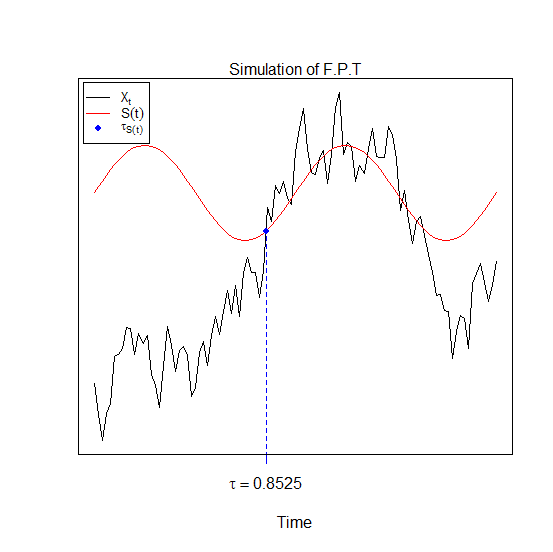
And dfptsde1d returns a kernel density approximation for \tau_{(X(t),S(t))} "first passage time".
with S(t) is through a continuous boundary (barrier).
An overview of this package, see browseVignettes('Sim.DiffProc') for more informations.
Value
dfptsde1d() |
gives the density estimate of fpt. |
fptsde1d() |
generates random of fpt. |
Author(s)
A.C. Guidoum, K. Boukhetala.
References
Argyrakisa, P. and G.H. Weiss (2006). A first-passage time problem for many random walkers. Physica A. 363, 343–347.
Aytug H., G. J. Koehler (2000). New stopping criterion for genetic algorithms. European Journal of Operational Research, 126, 662–674.
Boukhetala, K. (1996) Modelling and simulation of a dispersion pollutant with attractive centre. ed by Computational Mechanics Publications, Southampton ,U.K and Computational Mechanics Inc, Boston, USA, 245–252.
Boukhetala, K. (1998a). Estimation of the first passage time distribution for a simulated diffusion process. Maghreb Math.Rev, 7(1), 1–25.
Boukhetala, K. (1998b). Kernel density of the exit time in a simulated diffusion. les Annales Maghrebines De L ingenieur, 12, 587–589.
Ding, M. and G. Rangarajan. (2004). First Passage Time Problem: A Fokker-Planck Approach. New Directions in Statistical Physics. ed by L. T. Wille. Springer. 31–46.
Roman, R.P., Serrano, J. J., Torres, F. (2008). First-passage-time location function: Application to determine first-passage-time densities in diffusion processes. Computational Statistics and Data Analysis. 52, 4132–4146.
Roman, R.P., Serrano, J. J., Torres, F. (2012). An R package for an efficient approximation of first-passage-time densities for diffusion processes based on the FPTL function. Applied Mathematics and Computation, 218, 8408–8428.
Gardiner, C. W. (1997). Handbook of Stochastic Methods. Springer-Verlag, New York.
See Also
fptsde2d and fptsde3d simulation fpt for 2 and 3-dim SDE.
FPTL for computes values of the first passage time location (FPTL) function, and Approx.fpt.density
for approximate first-passage-time (f.p.t.) density in package "fptdApprox".
GQD.TIpassage for compute the First Passage Time Density of a GQD With Time Inhomogeneous Coefficients in package "DiffusionRgqd".
Examples
## Example 1: Ito SDE
## dX(t) = -4*X(t) *dt + 0.5*dW(t)
## S(t) = 0 (constant boundary)
set.seed(1234)
# SDE 1d
f <- expression( -4*x )
g <- expression( 0.5 )
mod <- snssde1d(drift=f,diffusion=g,x0=2,M=1000)
# boundary
St <- expression(0)
# random
out <- fptsde1d(mod, boundary=St)
out
summary(out)
# density approximate
den <- dfptsde1d(out)
den
plot(den)
## Example 2: Stratonovich SDE
## dX(t) = 0.5*X(t)*t *dt + sqrt(1+X(t)^2) o dW(t)
## S(t) = -0.5*sqrt(t) + exp(t^2) (time-dependent boundary)
set.seed(1234)
# SDE 1d
f <- expression( 0.5*x*t )
g <- expression( sqrt(1+x^2) )
mod2 <- snssde1d(drift=f,diffusion=g,x0=2,M=1000,type="srt")
# boundary
St <- expression(-0.5*sqrt(t)+exp(t^2))
# random
out2 <- fptsde1d(mod2,boundary=St)
out2
summary(out2)
# density approximate
plot(dfptsde1d(out2,bw='ucv'))
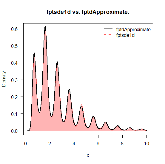
## Example 3: fptsde1d vs fptdApproximate
## Not run:
f <- expression( -0.5*x+0.5*5 )
g <- expression( 1 )
St <- expression(5+0.25*sin(2*pi*t))
mod <- snssde1d(drift=f,diffusion=g,boundary=St,x0=3,T=10,N=10^4,M =10000)
mod
# random
out3 <- fptsde1d(mod,boundary=St)
out3
summary(out3)
# density approximate:
library("fptdApprox")
# Under `fptdApprox':
# Define the diffusion process and give its transitional density:
OU <- diffproc(c("alpha*x + beta","sigma^2",
"dnorm((x-(y*exp(alpha*(t-s)) - beta*(1 - exp(alpha*(t-s)))/alpha))/
(sigma*sqrt((exp(2*alpha*(t-s)) - 1)/(2*alpha))),0,1)/
(sigma*sqrt((exp(2*alpha*(t-s)) - 1)/(2*alpha)))",
"pnorm(x, y*exp(alpha*(t-s)) - beta*(1 - exp(alpha*(t-s)))/alpha,
sigma*sqrt((exp(2*alpha*(t-s)) - 1)/(2*alpha)))"))
# Approximate the first passgage time density for OU, starting in X_0 = 3
# passing through 5+0.25*sin(2*pi*t) on the time interval [0,10]:
res <- Approx.fpt.density(OU, 0, 10, 3,"5+0.25*sin(2*pi*t)", list(alpha=-0.5,beta=0.5*5,sigma=1))
##
plot(dfptsde1d(out3,bw='ucv'),main = 'fptsde1d vs fptdApproximate')
lines(res$y~res$x, type = 'l',lwd=2)
legend('topright', lty = c('solid', 'dashed'), col = c(1, 2),
legend = c('fptdApproximate', 'fptsde1d'), lwd = 2, bty = 'n')
## End(Not run)
Approximate densities and random generation for first passage time in 2-D SDE's
Description
Kernel density and random generation for first-passage-time (f.p.t) in 2-dim stochastic differential equations.
Usage
fptsde2d(object, ...)
dfptsde2d(object, ...)

## Default S3 method:
fptsde2d(object, boundary, ...)
## S3 method for class 'fptsde2d'
summary(object, digits=NULL, ...)
## S3 method for class 'fptsde2d'
mean(x, ...)
## S3 method for class 'fptsde2d'
Median(x, ...)
## S3 method for class 'fptsde2d'
Mode(x, ...)
## S3 method for class 'fptsde2d'
quantile(x, ...)
## S3 method for class 'fptsde2d'
kurtosis(x, ...)
## S3 method for class 'fptsde2d'
skewness(x, ...)
## S3 method for class 'fptsde2d'
min(x, ...)
## S3 method for class 'fptsde2d'
max(x, ...)
## S3 method for class 'fptsde2d'
moment(x, ...)
## S3 method for class 'fptsde2d'
cv(x, ...)

## Default S3 method:
dfptsde2d(object, pdf=c("Joint","Marginal"), ...)
## S3 method for class 'dfptsde2d'
plot(x,display=c("persp","rgl","image","contour"),
                         hist=FALSE, ...)
Arguments
object |
an object inheriting from class |
boundary |
an |
pdf |
probability density function |
x |
an object inheriting from class |
digits |
integer, used for number formatting. |
display |
display plots. |
hist |
if |
... |
potentially further arguments for (non-default) methods. arguments to be passed to methods, such as |
Details
The function fptsde1d returns a random variable (\tau_{(X(t),S(t))},\tau_{(Y(t),S(t))}) "first passage time", is defined as :
\tau_{(X(t),S(t))} = \{ t \geq 0 ; X_{t} \geq S(t) \},\quad if \quad X(t_{0}) < S(t_{0})
\tau_{(Y(t),S(t))} = \{ t \geq 0 ; Y_{t} \geq S(t) \},\quad if \quad Y(t_{0}) < S(t_{0})
and:
\tau_{(X(t),S(t))} = \{ t \geq 0 ; X_{t} \leq S(t) \},\quad if \quad X(t_{0}) > S(t_{0})
\tau_{(Y(t),S(t))} = \{ t \geq 0 ; Y_{t} \leq S(t) \},\quad if \quad Y(t_{0}) > S(t_{0})
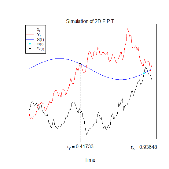
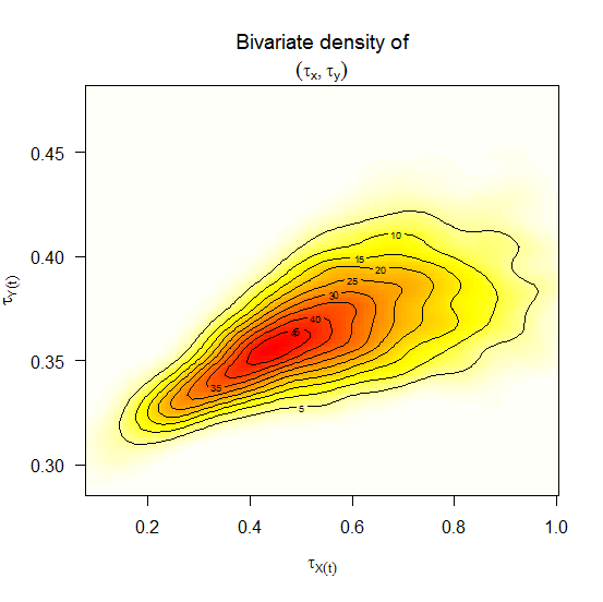
And dfptsde2d returns a kernel density approximation for (\tau_{(X(t),S(t))},\tau_{(Y(t),S(t))}) "first passage time".
with S(t) is through a continuous boundary (barrier).
An overview of this package, see browseVignettes('Sim.DiffProc') for more informations.
Value
dfptsde2d() |
gives the kernel density approximation for fpt. |
fptsde2d() |
generates random of fpt. |
Author(s)
A.C. Guidoum, K. Boukhetala.
References
Argyrakisa, P. and G.H. Weiss (2006). A first-passage time problem for many random walkers. Physica A. 363, 343–347.
Aytug H., G. J. Koehler (2000). New stopping criterion for genetic algorithms. European Journal of Operational Research, 126, 662–674.
Boukhetala, K. (1996) Modelling and simulation of a dispersion pollutant with attractive centre. ed by Computational Mechanics Publications, Southampton ,U.K and Computational Mechanics Inc, Boston, USA, 245–252.
Boukhetala, K. (1998a). Estimation of the first passage time distribution for a simulated diffusion process. Maghreb Math.Rev, 7(1), 1–25.
Boukhetala, K. (1998b). Kernel density of the exit time in a simulated diffusion. les Annales Maghrebines De L ingenieur, 12, 587–589.
Ding, M. and G. Rangarajan. (2004). First Passage Time Problem: A Fokker-Planck Approach. New Directions in Statistical Physics. ed by L. T. Wille. Springer. 31–46.
Roman, R.P., Serrano, J. J., Torres, F. (2008). First-passage-time location function: Application to determine first-passage-time densities in diffusion processes. Computational Statistics and Data Analysis. 52, 4132–4146.
Roman, R.P., Serrano, J. J., Torres, F. (2012). An R package for an efficient approximation of first-passage-time densities for diffusion processes based on the FPTL function. Applied Mathematics and Computation, 218, 8408–8428.
Gardiner, C. W. (1997). Handbook of Stochastic Methods. Springer-Verlag, New York.
See Also
fptsde1d for simulation fpt in sde 1-dim. fptsde3d for simulation fpt in sde 3-dim.
FPTL for computes values of the first passage time location (FPTL) function, and Approx.fpt.density
for approximate first-passage-time (f.p.t.) density in package "fptdApprox".
GQD.TIpassage for compute the First Passage Time Density of a GQD With Time Inhomogeneous Coefficients in package "DiffusionRgqd".
Examples
## dX(t) = 5*(-1-Y(t))*X(t) * dt + 0.5 * dW1(t)
## dY(t) = 5*(-1-X(t))*Y(t) * dt + 0.5 * dW2(t)
## x0 = 2, y0 = -2, and barrier -3+5*t.
## W1(t) and W2(t) two independent Brownian motion
set.seed(1234)

# SDE's 2d
fx <- expression(5*(-1-y)*x , 5*(-1-x)*y)
gx <- expression(0.5 , 0.5)
mod2d <- snssde2d(drift=fx,diffusion=gx,x0=c(2,-2),M=100)

# boundary

St <- expression(-1+5*t)

# random fpt

out <- fptsde2d(mod2d,boundary=St)
out
summary(out)

# Marginal density

denM <- dfptsde2d(out,pdf="M")
denM
plot(denM)

# Joint density

denJ <- dfptsde2d(out,pdf="J",n=200,lims=c(0.28,0.4,0.04,0.13))
denJ
plot(denJ)
plot(denJ,display="image")
plot(denJ,display="image",drawpoints=TRUE,cex=0.5,pch=19,col.pt='green')
plot(denJ,display="contour")
plot(denJ,display="contour",color.palette=colorRampPalette(c('white','green','blue','red')))
Approximate densities and random generation for first passage time in 3-D SDE's
Description
Kernel density and random generation for first-passage-time (f.p.t) in 3-dim stochastic differential equations.
Usage
fptsde3d(object, ...)
dfptsde3d(object, ...)

## Default S3 method:
fptsde3d(object, boundary, ...)
## S3 method for class 'fptsde3d'
summary(object, digits=NULL, ...)
## S3 method for class 'fptsde3d'
mean(x, ...)
## S3 method for class 'fptsde3d'
Median(x, ...)
## S3 method for class 'fptsde3d'
Mode(x, ...)
## S3 method for class 'fptsde3d'
quantile(x, ...)
## S3 method for class 'fptsde3d'
kurtosis(x, ...)
## S3 method for class 'fptsde3d'
skewness(x, ...)
## S3 method for class 'fptsde3d'
min(x, ...)
## S3 method for class 'fptsde3d'
max(x, ...)
## S3 method for class 'fptsde3d'
moment(x, ...)
## S3 method for class 'fptsde3d'
cv(x, ...)

## Default S3 method:
dfptsde3d(object, pdf=c("Joint","Marginal"), ...)
## S3 method for class 'dfptsde3d'
plot(x,display="rgl",hist=FALSE, ...)
Arguments
object |
an object inheriting from class |
boundary |
an |
pdf |
probability density function |
x |
an object inheriting from class |
digits |
integer, used for number formatting. |
display |
display plots. |
hist |
if |
... |
potentially arguments to be passed to methods, such as |
Details
The function fptsde3d returns a random variable (\tau_{(X(t),S(t))},\tau_{(Y(t),S(t))},\tau_{(Z(t),S(t))}) "first passage time", is defined as :
\tau_{(X(t),S(t))} = \{ t \geq 0 ; X_{t} \geq S(t) \},\quad if \quad X(t_{0}) < S(t_{0})
\tau_{(Y(t),S(t))} = \{ t \geq 0 ; Y_{t} \geq S(t) \},\quad if \quad Y(t_{0}) < S(t_{0})
\tau_{(Z(t),S(t))} = \{ t \geq 0 ; Z_{t} \geq S(t) \},\quad if \quad Z(t_{0}) < S(t_{0})
and:
\tau_{(X(t),S(t))} = \{ t \geq 0 ; X_{t} \leq S(t) \},\quad if \quad X(t_{0}) > S(t_{0})
\tau_{(Y(t),S(t))} = \{ t \geq 0 ; Y_{t} \leq S(t) \},\quad if \quad Y(t_{0}) > S(t_{0})
\tau_{(Z(t),S(t))} = \{ t \geq 0 ; Z_{t} \leq S(t) \},\quad if \quad Z(t_{0}) > S(t_{0})
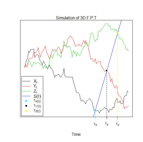
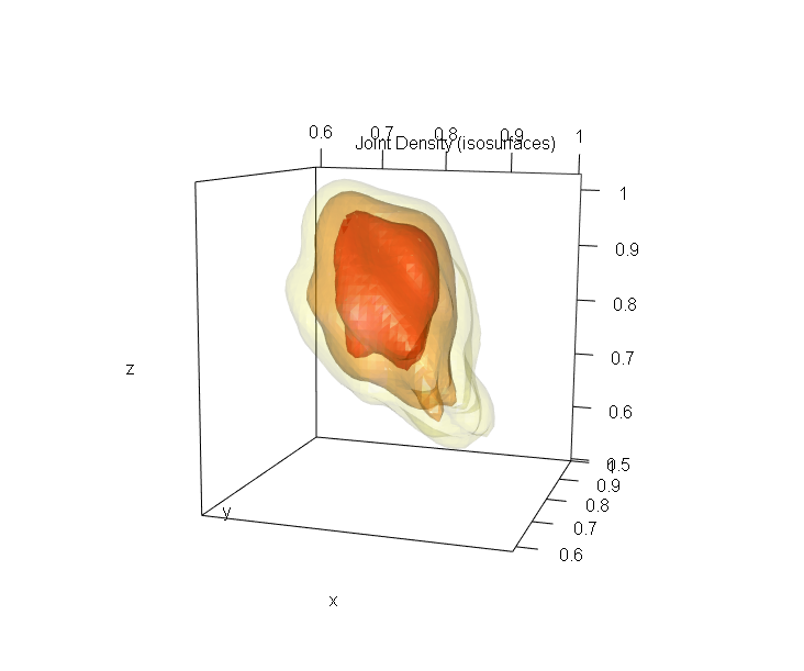
And dfptsde3d returns a marginal kernel density approximation for (\tau_{(X(t),S(t))},\tau_{(Y(t),S(t))},\tau_{(Z(t),S(t))}) "first passage time".
with S(t) is through a continuous boundary (barrier).
An overview of this package, see browseVignettes('Sim.DiffProc') for more informations.
Value
dfptsde3d() |
gives the marginal kernel density approximation for fpt. |
fptsde3d() |
generates random of fpt. |
Author(s)
A.C. Guidoum, K. Boukhetala.
References
Argyrakisa, P. and G.H. Weiss (2006). A first-passage time problem for many random walkers. Physica A. 363, 343–347.
Aytug H., G. J. Koehler (2000). New stopping criterion for genetic algorithms. European Journal of Operational Research, 126, 662–674.
Boukhetala, K. (1996) Modelling and simulation of a dispersion pollutant with attractive centre. ed by Computational Mechanics Publications, Southampton ,U.K and Computational Mechanics Inc, Boston, USA, 245–252.
Boukhetala, K. (1998a). Estimation of the first passage time distribution for a simulated diffusion process. Maghreb Math.Rev, 7(1), 1–25.
Boukhetala, K. (1998b). Kernel density of the exit time in a simulated diffusion. les Annales Maghrebines De L ingenieur, 12, 587–589.
Ding, M. and G. Rangarajan. (2004). First Passage Time Problem: A Fokker-Planck Approach. New Directions in Statistical Physics. ed by L. T. Wille. Springer. 31–46.
Roman, R.P., Serrano, J. J., Torres, F. (2008). First-passage-time location function: Application to determine first-passage-time densities in diffusion processes. Computational Statistics and Data Analysis. 52, 4132–4146.
Roman, R.P., Serrano, J. J., Torres, F. (2012). An R package for an efficient approximation of first-passage-time densities for diffusion processes based on the FPTL function. Applied Mathematics and Computation, 218, 8408–8428.
Gardiner, C. W. (1997). Handbook of Stochastic Methods. Springer-Verlag, New York.
See Also
fptsde1d for simulation fpt in sde 1-dim. fptsde2d for simulation fpt in sde 2-dim.
FPTL for computes values of the first passage time location (FPTL) function, and Approx.fpt.density
for approximate first-passage-time (f.p.t.) density in package "fptdApprox".
GQD.TIpassage for compute the First Passage Time Density of a GQD With Time Inhomogeneous Coefficients in package "DiffusionRgqd".
Examples
## dX(t) = 4*(-1-X(t))*Y(t) dt + 0.2 * dW1(t)
## dY(t) = 4*(1-Y(t)) *X(t) dt + 0.2 * dW2(t)
## dZ(t) = 4*(1-Z(t)) *Y(t) dt + 0.2 * dW3(t)
## x0 = 0, y0 = -2, z0 = 0, and barrier -3+5*t.
## W1(t), W2(t) and W3(t) three independent Brownian motion
set.seed(1234)

# SDE's 3d

fx <- expression(4*(-1-x)*y, 4*(1-y)*x, 4*(1-z)*y)
gx <- rep(expression(0.2),3)
mod3d <- snssde3d(drift=fx,diffusion=gx,M=500)

# boundary
St <- expression(-3+5*t)

# random

out <- fptsde3d(mod3d,boundary=St)
out
summary(out)

# Marginal density

denM <- dfptsde3d(out,pdf="M")
denM
plot(denM)

# Multiple isosurfaces
## Not run:
denJ <- dfptsde3d(out,pdf="J")
denJ
plot(denJ,display="rgl")

## End(Not run)
Monte-Carlo statistics of SDE's
Description
Generic function for compute the kurtosis, skewness, median, mode and coefficient of variation (relative variability), moment and confidence interval of class "sde".
Usage
## Default S3 method:
bconfint(x, level = 0.95, ...)
## Default S3 method:
kurtosis(x, ...)
## Default S3 method:
moment(x, order = 1,center = TRUE, ...)
## Default S3 method:
cv(x, ...)
## Default S3 method:
skewness(x, ...)
## Default S3 method:
Median(x, ...)
## Default S3 method:
Mode(x, ...)
Arguments
x |
an object inheriting from class |
order |
order of moment. |
center |
if |
level |
the confidence level required. |
... |
potentially further arguments for (non-default) methods. |
Author(s)
A.C. Guidoum, K. Boukhetala.
Examples
## Example 1:
## dX(t) = 2*(3-X(t)) *dt + dW(t)
set.seed(1234)

f <- expression( 2*(3-x) )
g <- expression( 1 )
mod <- snssde1d(drift=f,diffusion=g,M=10000,T=5)
## Monte-Carlo statistics of 5000 trajectory of X(t) at final time T of 'mod'
summary(mod)
kurtosis(mod)
skewness(mod)
mean(mod)
Median(mod)
Mode(mod)
moment(mod,order=4)
cv(mod)
bconfint(mod,level = 0.95) ## of mean
Plotting for Class SDE
Description
Generic function for plotting.
Usage
## Default S3 method:
plot2d(x, ...)
## Default S3 method:
lines2d(x, ...)
## Default S3 method:
points2d(x, ...)
## Default S3 method:
plot3D(x, display = c("persp","rgl"), ...)
Arguments
x |
an object inheriting from class |
display |
|
... |
other graphics parameters, see |
Details
The 2 and 3-dim plot of class sde.
Author(s)
A.C. Guidoum, K. Boukhetala.
Examples
## Example 1:
set.seed(1234)

fx <- rep(expression(0),2)
gx <- rep(expression(1),2)

res <- snssde2d(drift=fx,diffusion=gx,N=5000)
plot2d(res,type="l")
Approximate transitional densities and random generation for 1-D SDE
Description
Transition density and random generation for X(t-s) | X(s)=x0 of the 1-dim SDE.
Usage
rsde1d(object, ...)
dsde1d(object, ...)

## Default S3 method:
rsde1d(object, at, ...)

## Default S3 method:
dsde1d(object, at, ...)
## S3 method for class 'dsde1d'
plot(x,hist=FALSE, ...)
Arguments
object |
an object inheriting from class |
at |
time between |
x |
an object inheriting from class |
hist |
if |
... |
potentially arguments to be passed to methods, such as |
Details
The function rsde1d returns a M random variable x_{t=at} realize at time t=at defined by :
x_{ t=at } = \{ t \geq 0 ; x = X_{ t=at } \}
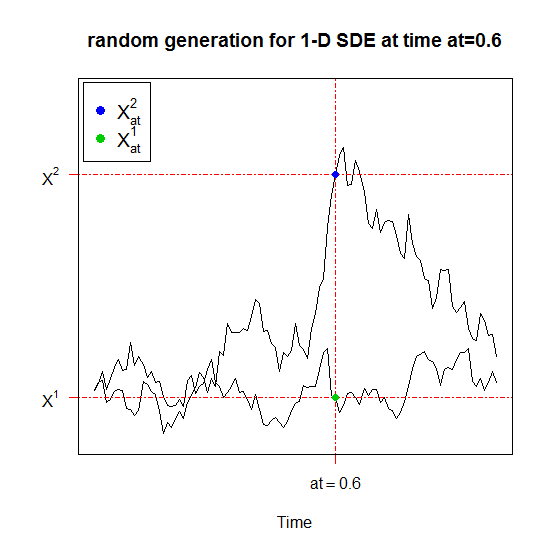
And dsde1d returns a transition density approximation for X(t-s) | X(s)=x0.
with t= at is a fixed time between t0 and T.
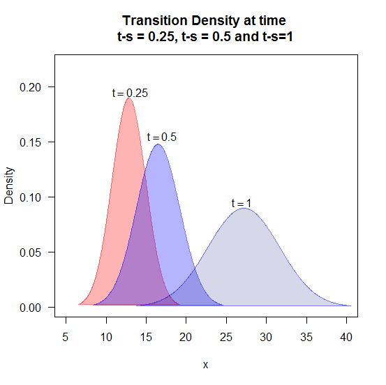
An overview of this package, see browseVignettes('Sim.DiffProc') for more informations.
Value
dsde1d() |
gives the transition density estimate of |
rsde1d() |
generates random of |
Author(s)
A.C. Guidoum, K. Boukhetala.
See Also
density Kernel density estimation in "stats" package.
kde Kernel density estimate for 1- to 6-dimensional data in "ks" package.
sm.density Nonparametric density estimation in one, two or three dimensions in "sm" package.
rng random number generators in "yuima" package.
dcSim Pedersen's simulated transition density in "sde" package.
rcBS, rcCIR, rcOU and rsOU in package "sde".
dcBS, dcCIR, dcOU and dsOU in package "sde".
GQD.density Generate the transition density of a scalar generalized quadratic diffusion in "DiffusionRgqd" package.
Examples
## Example 1:
## dX(t) = (-2*(X(t)<=0)+2*(X(t)>=0)) *dt + 0.5 * dW(t)
set.seed(1234)

f <- expression(-2*(x<=0)+2*(x>=0))
g <- expression(0.5)
res1 <- snssde1d(drift=f,diffusion=g,M=5000)
x <- rsde1d(res1, at = 1)
summary(x)
dens1 <-  dsde1d(res1, at = 1)
dens1
plot(dens1,main="Transition density of X(t=1)|X(s=0)=0") # kernel estimated
plot(dens1,hist=TRUE) # histogramme

## Example 2:
## Transition density of standard Brownian motion W(t) at time = 0.5
set.seed(1234)

f <- expression(0)
g <- expression(1)
res2 <- snssde1d(drift=f,diffusion=g,M=5000)
plot(dsde1d(res2, at = 0.5),dens=function(x) dnorm(x,0,sqrt(0.5)))
plot(dsde1d(res2, at = 0.5),dens=function(x) dnorm(x,0,sqrt(0.5)),hist=TRUE)

## Example 3: Transition density of Brownian motion W(t) in [0,1]

## Not run:
for (i in seq(res2$t0,res2$T,by=res2$Dt)){
plot(dsde1d(res2, at = i),main=paste0('Transition Density \n t = ',i))
}

## End(Not run)

## Example 4:
## Transition density of bridge Brownian motion W(t) at time = 0.25 and 0.75
set.seed(1234)
## Not run:
f <- expression(0)
g <- expression(1)
Bd <- bridgesde1d(drift=f,diffusion=g,M=5000)
Bd
plot(dsde1d(Bd, at = 0.25))         ## Transition Density at time=0.25
plot(dsde1d(Bd, at = 0.75),add=TRUE)## Transition Density at time=0.75

## End(Not run)
Approximate transitional densities and random generation for 2-D SDE's
Description
Transition density and random generation for the joint and marginal of (X(t-s),Y(t-s) | X(s)=x0,Y(s)=y0) of the SDE's 2-d.
Usage
rsde2d(object, ...)
dsde2d(object, ...)

## Default S3 method:
rsde2d(object, at, ...)

## Default S3 method:
dsde2d(object, pdf=c("Joint","Marginal"), at, ...)
## S3 method for class 'dsde2d'
plot(x,display=c("persp","rgl","image","contour"),hist=FALSE,...)
Arguments
object |
an object inheriting from class |
at |
time between |
pdf |
probability density function |
x |
an object inheriting from class |
display |
display plots. |
hist |
if |
... |
potentially potentially arguments to be passed to methods, such as |
Details
The function rsde2d returns a M random variable x_{t=at},y_{t=at} realize at time t=at.
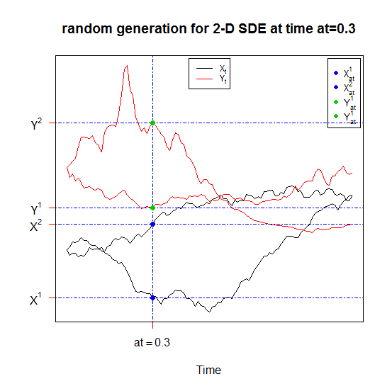
And dsde2d returns a bivariate density approximation for (X(t-s),Y(t-s) | X(s)=x0,Y(s)=y0). with t=at is a fixed time between t0 and T.
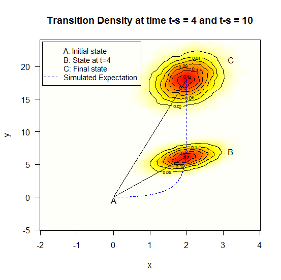
An overview of this package, see browseVignettes('Sim.DiffProc') for more informations.
Value
dsde2d() |
gives the bivariate density approximation for |
rsde2d() |
generates random of the couple |
Author(s)
A.C. Guidoum, K. Boukhetala.
See Also
kde2d Two-dimensional kernel density estimation in "MASS" package.
kde Kernel density estimate for 1- to 6-dimensional data in "ks" package.
sm.density Nonparametric density estimation in one, two or three dimensions in "sm" package.
rng random number generators in "yuima" package.
BiGQD.density Generate the transition density of a bivariate generalized quadratic diffusion model (2D GQD) in "DiffusionRgqd" package.
Examples
## Example:1
set.seed(1234)

# SDE's 2d
fx <- expression(3*(2-y),2*x)
gx <- expression(1,y)
mod2d <- snssde2d(drift=fx,diffusion=gx,x0=c(1,2),M=1000)

# random
r2d <- rsde2d(mod2d,at=0.5)
summary(r2d)

# Marginal density

denM <- dsde2d(mod2d,pdf="M", at=0.5)
denM
plot(denM)

# Joint density
denJ <- dsde2d(mod2d,pdf="J",n=200, at= 0.5,lims=c(-3,4,0,6))
denJ
plot(denJ)
plot(denJ,display="contour")

## Example 2: Bivariate Transition Density of 2 Brownian motion (W1(t),W2(t)) in [0,1]

## Not run:
B2d <- snssde2d(drift=rep(expression(0),2),diffusion=rep(expression(1),2),
       M=10000)
for (i in seq(B2d$Dt,B2d$T,by=B2d$Dt)){
plot(dsde2d(B2d, at = i,lims=c(-3,3,-3,3),n=100),
   display="contour",main=paste0('Transition Density \n t = ',i))
}

## End(Not run)

## Example 3:

## Not run:
fx <- expression(4*(-1-x)*y , 4*(1-y)*x )
gx <- expression(0.25*y,0.2*x)
mod2d1 <- snssde2d(drift=fx,diffusion=gx,x0=c(x0=1,y0=-1),
      M=5000,type="str")

# Marginal transition density
for (i in seq(mod2d1$Dt,mod2d1$T,by=mod2d1$Dt)){
plot(dsde2d(mod2d1,pdf="M", at = i),main=
      paste0('Marginal Transition Density \n t = ',i))
}

# Bivariate transition density
for (i in seq(mod2d1$Dt,mod2d1$T,by=mod2d1$Dt)){
plot(dsde2d(mod2d1, at = i,lims=c(-1,2,-1,1),n=100),
    display="contour",main=paste0('Transition Density \n t = ',i))
}

## End(Not run)

## Example 4: Bivariate Transition Density of 2 bridge Brownian motion (W1(t),W2(t)) in [0,1]

## Not run:
B2d <- bridgesde2d(drift=rep(expression(0),2),
  diffusion=rep(expression(1),2),M=5000)
for (i in seq(0.01,0.99,by=B2d$Dt)){
plot(dsde2d(B2d, at = i,lims=c(-3,3,-3,3),
 n=100),display="contour",main=
 paste0('Transition Density \n t = ',i))
}

## End(Not run)

## Example 5: Bivariate Transition Density of bridge
## Ornstein-Uhlenbeck process and its integral in [0,5]
## dX(t) = 4*(-1-X(t)) dt + 0.2 dW1(t)
## dY(t) = X(t) dt + 0 dW2(t)
## x01 = 0 , y01 = 0
## x02 = 0, y02 = 0
## Not run:
fx <- expression(4*(-1-x) , x)
gx <- expression(0.2 , 0)
OUI <- bridgesde2d(drift=fx,diffusion=gx,Dt=0.005,M=1000)
for (i in seq(0.01,4.99,by=OUI$Dt)){
plot(dsde2d(OUI, at = i,lims=c(-1.2,0.2,-2.5,0.2),n=100),
 display="contour",main=paste0('Transition Density \n t = ',i))
}

## End(Not run)
Approximate transitional densities and random generation for 3-D SDE's
Description
Transition density and random generation for the joint and marginal of (X(t-s),Y(t-s),Z(t-s) | X(s)=x0,Y(s)=y0,Z(s)=z0) of the SDE's 3-d.
Usage
rsde3d(object, ...)
dsde3d(object, ...)

## Default S3 method:
rsde3d(object, at, ...)

## Default S3 method:
dsde3d(object, pdf=c("Joint","Marginal"), at, ...)
## S3 method for class 'dsde3d'
plot(x,display="rgl",hist=FALSE,...)
Arguments
object |
an object inheriting from class |
at |
time between |
pdf |
probability density function |
x |
an object inheriting from class |
display |
display plots. |
hist |
if |
... |
potentially arguments to be passed to methods, such as |
Details
The function rsde3d returns a M random variable x_{t=at},y_{t=at},z_{t=at} realize at time t=at.
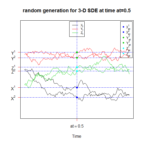
And dsde3d returns a trivariate kernel density approximation for (X(t-s),Y(t-s),Z(t-s) | X(s)=x0,Y(s)=y0,Z(s)=z0). with t= at is a fixed time between t0 and T.
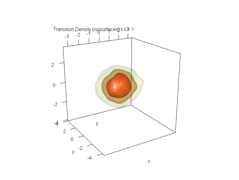
An overview of this package, see browseVignettes('Sim.DiffProc') for more informations.
Value
dsde3d() |
gives the trivariate density approximation |
rsde3d() |
generates random of the |
Author(s)
A.C. Guidoum, K. Boukhetala.
See Also
kde Kernel density estimate for 1- to 6-dimensional data in "ks" package.
sm.density Nonparametric density estimation in one, two or three dimensions in "sm" package.
kde3d Compute a three dimension kernel density estimate in "misc3d" package.
rng random number generators in "yuima" package.
rcBS, rcCIR, rcOU and rsOU in package "sde".
Examples
## Example 1: Ito sde
## dX(t) = (2*(Y(t)>0)-2*(Z(t)<=0)) dt + 0.2 * dW1(t)
## dY(t) = -2*Y(t) dt + 0.2 * dW2(t)
## dZ(t) = -2*Z(t) dt + 0.2 * dW3(t)
## W1(t), W2(t) and W3(t) three independent Brownian motion
set.seed(1234)
fx <- expression(2*(y>0)-2*(z<=0) , -2*y, -2*z)
gx <- rep(expression(0.2),3)
mod3d1 <- snssde3d(x0=c(0,2,-2),drift=fx,diffusion=gx,M=1000,Dt=0.003)

# random at t= 0.75
r3d1 <- rsde3d(mod3d1,at=0.75)
summary(r3d1)

# Marginal transition density at t=0.75, t0=0

denM <- dsde3d(mod3d1,pdf="M",at=0.75)
denM
plot(denM)

# for Joint transition density at t=0.75;t0=0
# Multiple isosurfaces
## Not run:
denJ <- dsde3d(mod3d1,pdf="J", at= 0.75)
denJ
plot(denJ,display="rgl")

## End(Not run)

## Example 2: Stratonovich sde
## dX(t) = Y(t)* dt + X(t) o dW1(t)
## dY(t) = (4*( 1-X(t)^2 )* Y(t) - X(t))* dt + 0.2 o dW2(t)
## dZ(t) = (4*( 1-X(t)^2 )* Z(t) - X(t))* dt + 0.2 o dW3(t)
set.seed(1234)

fx <- expression( y , (4*( 1-x^2 )* y - x), (4*( 1-x^2 )* z - x))
gx <- expression( x , 0.2, 0.2)
mod3d2 <- snssde3d(drift=fx,diffusion=gx,M=1000,type="str")

# random
r3d2 <- rsde3d(mod3d2)
summary(r3d2)

# Marginal transition density at t=1, t0=0

denM <- dsde3d(mod3d2,pdf="M")
denM
plot(denM)

# for Joint transition density at t=1;t0=0
# Multiple isosurfaces
## Not run:
denJ <- dsde3d(mod3d2,pdf="J")
denJ
plot(denJ,display="rgl")

## End(Not run)

## Example 3: Tivariate Transition Density of 3 Brownian motion (W1(t),W2(t),W3(t)) in [0,1]

## Not run:
B3d <- snssde3d(drift=rep(expression(0),3),diffusion=rep(expression(1),3),M=500)
for (i in seq(B3d$Dt,B3d$T,by=B3d$Dt)){
plot(dsde3d(B3d, at = i,pdf="J"),box=F,main=paste0('Transition Density t = ',i))
}

## End(Not run)
Simulation of 1-D Stochastic Differential Equation
Description
The (S3) generic function snssde1d of simulation of solution to 1-dim stochastic differential equation of Itô or Stratonovich type, with different methods.
Usage
snssde1d(N, ...)
## Default S3 method:
snssde1d(N = 1000, M = 1, x0 = 0, t0 = 0, T = 1, Dt,
   drift, diffusion, alpha = 0.5, mu = 0.5, type = c("ito", "str"),
   method = c("euler", "milstein", "predcorr", "smilstein", "taylor",
   "heun", "rk1", "rk2", "rk3"), ...)

## S3 method for class 'snssde1d'
summary(object, at ,digits=NULL, ...)
## S3 method for class 'snssde1d'
time(x, ...)
## S3 method for class 'snssde1d'
mean(x, at, ...)
## S3 method for class 'snssde1d'
Median(x, at, ...)
## S3 method for class 'snssde1d'
Mode(x, at, ...)
## S3 method for class 'snssde1d'
quantile(x, at, ...)
## S3 method for class 'snssde1d'
kurtosis(x, at, ...)
## S3 method for class 'snssde1d'
min(x, at, ...)
## S3 method for class 'snssde1d'
max(x, at, ...)
## S3 method for class 'snssde1d'
skewness(x, at, ...)
## S3 method for class 'snssde1d'
moment(x, at,  ...)
## S3 method for class 'snssde1d'
cv(x, at,  ...)
## S3 method for class 'snssde1d'
bconfint(x, at,  ...)

## S3 method for class 'snssde1d'
plot(x, ...)
## S3 method for class 'snssde1d'
lines(x, ...)
## S3 method for class 'snssde1d'
points(x, ...)
Arguments
N |
number of simulation steps. |
M |
number of trajectories (Monte-Carlo). |
x0 |
initial value of the process at time |
t0 |
initial time. |
T |
ending time. |
Dt |
time step of the simulation (discretization). If it is |
drift |
drift coefficient: an |
diffusion |
diffusion coefficient: an |
alpha, mu |
weight of the predictor-corrector scheme; the default |
type |
if |
method |
numerical methods of simulation, the default |
x, object |
an object inheriting from class |
at |
time between |
digits |
integer, used for number formatting. |
... |
potentially further arguments for (non-default) methods. |
Details
The function snssde1d returns a ts x of length N+1; i.e. solution of the sde of Ito or
Stratonovich types; If Dt is not specified, then the best discretization \Delta t = \frac{T-t_{0}}{N}.
The Ito stochastic differential equation is:
dX(t) = a(t,X(t)) dt + b(t,X(t)) dW(t)
Stratonovich sde :
dX(t) = a(t,X(t)) dt + b(t,X(t)) \circ dW(t)
The methods of approximation are classified according to their different properties. Mainly two criteria of optimality are used in the literature: the strong
and the weak (orders of) convergence. The method of simulation can be one among: Euler-Maruyama Order 0.5, Milstein Order 1, Milstein Second-Order,
Predictor-Corrector method, Itô-Taylor Order 1.5, Heun Order 2 and Runge-Kutta Order 1, 2 and 3.
An overview of this package, see browseVignettes('Sim.DiffProc') for more informations.
Value
snssde1d returns an object inheriting from class "snssde1d".
X |
an invisible |
drift |
drift coefficient. |
diffusion |
diffusion coefficient. |
type |
type of sde. |
method |
the numerical method used. |
Author(s)
A.C. Guidoum, K. Boukhetala.
References
Guidoum AC, Boukhetala K (2020). "Performing Parallel Monte Carlo and Moment Equations Methods for Itô and Stratonovich Stochastic Differential Systems: R Package Sim.DiffProc". Journal of Statistical Software, 96(2), 1–82. doi:10.18637/jss.v096.i02
Friedman, A. (1975). Stochastic differential equations and applications. Volume 1, ACADEMIC PRESS.
Henderson, D. and Plaschko,P. (2006). Stochastic differential equations in science and engineering. World Scientific.
Allen, E. (2007). Modeling with Ito stochastic differential equations. Springer-Verlag.
Jedrzejewski, F. (2009). Modeles aleatoires et physique probabiliste. Springer-Verlag.
Iacus, S.M. (2008). Simulation and inference for stochastic differential equations: with R examples. Springer-Verlag, New York.
Kloeden, P.E, and Platen, E. (1989). A survey of numerical methods for stochastic differential equations. Stochastic Hydrology and Hydraulics, 3, 155–178.
Kloeden, P.E, and Platen, E. (1991a). Relations between multiple ito and stratonovich integrals. Stochastic Analysis and Applications, 9(3), 311–321.
Kloeden, P.E, and Platen, E. (1991b). Stratonovich and ito stochastic taylor expansions. Mathematische Nachrichten, 151, 33–50.
Kloeden, P.E, and Platen, E. (1995). Numerical Solution of Stochastic Differential Equations. Springer-Verlag, New York.
Oksendal, B. (2000). Stochastic Differential Equations: An Introduction with Applications. 5th edn. Springer-Verlag, Berlin.
Platen, E. (1980). Weak convergence of approximations of ito integral equations. Z Angew Math Mech. 60, 609–614.
Platen, E. and Bruti-Liberati, N. (2010). Numerical Solution of Stochastic Differential Equations with Jumps in Finance. Springer-Verlag, New York
Saito, Y, and Mitsui, T. (1993). Simulation of Stochastic Differential Equations. The Annals of the Institute of Statistical Mathematics, 3, 419–432.
See Also
snssde2d and snssde3d for 2 and 3-dim sde.
sde.sim in package "sde".
simulate in package "yuima".
Examples
## Example 1: Ito sde
## dX(t) = 2*(3-X(t)) dt + 2*X(t) dW(t)
set.seed(1234)

f <- expression(2*(3-x) )
g <- expression(1)
mod1 <- snssde1d(drift=f,diffusion=g,M=4000,x0=10,Dt=0.01)
mod1
summary(mod1)
## Not run:
plot(mod1)
lines(time(mod1),apply(mod1$X,1,mean),col=2,lwd=2)
lines(time(mod1),apply(mod1$X,1,bconfint,level=0.95)[1,],col=4,lwd=2)
lines(time(mod1),apply(mod1$X,1,bconfint,level=0.95)[2,],col=4,lwd=2)
legend("topright",c("mean path",paste("bound of", 95," percent confidence")),
       inset = .01,col=c(2,4),lwd=2,cex=0.8)

## End(Not run)
## Example 2: Stratonovich sde
## dX(t) = ((2-X(t))/(2-t)) dt + X(t) o dW(t)
set.seed(1234)

f <- expression((2-x)/(2-t))
g <- expression(x)
mod2 <- snssde1d(type="str",drift=f,diffusion=g,M=4000,x0=1, method="milstein")
mod2
summary(mod2,at = 0.25)
summary(mod2,at = 1)
## Not run:
plot(mod2)
lines(time(mod2),apply(mod2$X,1,mean),col=2,lwd=2)
lines(time(mod2),apply(mod2$X,1,bconfint,level=0.95)[1,],col=4,lwd=2)
lines(time(mod2),apply(mod2$X,1,bconfint,level=0.95)[2,],col=4,lwd=2)
legend("topleft",c("mean path",paste("bound of", 95," percent confidence")),
       inset = .01,col=c(2,4),lwd=2,cex=0.8)

## End(Not run)
Simulation of 2-D Stochastic Differential Equation
Description
The (S3) generic function snssde2d of simulation of solutions to 2-dim stochastic differential equations of Itô or Stratonovich type, with different methods.
Usage
snssde2d(N, ...)
## Default S3 method:
snssde2d(N = 1000, M = 1, x0 = c(0,0),t0 = 0, T = 1, Dt,
   drift, diffusion, corr = NULL, type = c("ito", "str"), alpha = 0.5, mu = 0.5,
   method = c("euler", "milstein", "predcorr", "smilstein", "taylor",
   "heun", "rk1", "rk2","rk3"), ...)

## S3 method for class 'snssde2d'
summary(object, at, digits=NULL,...)
## S3 method for class 'snssde2d'
time(x, ...)
## S3 method for class 'snssde2d'
mean(x, at, ...)
## S3 method for class 'snssde2d'
Median(x, at, ...)
## S3 method for class 'snssde2d'
Mode(x, at, ...)
## S3 method for class 'snssde2d'
quantile(x, at, ...)
## S3 method for class 'snssde2d'
kurtosis(x, at, ...)
## S3 method for class 'snssde2d'
skewness(x, at, ...)
## S3 method for class 'snssde2d'
min(x, at, ...)
## S3 method for class 'snssde2d'
max(x, at, ...)
## S3 method for class 'snssde2d'
moment(x, at, ...)
## S3 method for class 'snssde2d'
cv(x, at, ...)
## S3 method for class 'snssde2d'
bconfint(x, at, ...)

## S3 method for class 'snssde2d'
plot(x, ...)
## S3 method for class 'snssde2d'
lines(x, ...)
## S3 method for class 'snssde2d'
points(x, ...)
## S3 method for class 'snssde2d'
plot2d(x, ...)
## S3 method for class 'snssde2d'
lines2d(x, ...)
## S3 method for class 'snssde2d'
points2d(x, ...)
Arguments
N |
number of simulation steps. |
M |
number of trajectories (Monte-Carlo). |
x0 |
initial values x0=(x,y) of the process |
t0 |
initial time. |
T |
ending time. |
Dt |
time step of the simulation (discretization). If it is |
drift |
drift coefficient: an |
diffusion |
diffusion coefficient: an |
corr |
the correlation structure of two Brownian motions W1(t) and W2(t); must be a real symmetric positive-definite square matrix of dimension 2. |
type |
if |
alpha, mu |
weight of the predictor-corrector scheme; the default |
method |
numerical methods of simulation, the default |
x, object |
an object inheriting from class |
at |
time between |
digits |
integer, used for number formatting. |
... |
potentially further arguments for (non-default) methods. |
Details
The function snssde2d returns a mts x of length N+1; i.e. solution of the 2-dim sde (X_{t},Y_{t})
of Ito or Stratonovich types; If Dt is not specified, then the best discretization \Delta t = \frac{T-t_{0}}{N}.
The 2-dim Ito stochastic differential equation is:
dX(t) = a(t,X(t),Y(t)) dt + b(t,X(t),Y(t)) dW_{1}(t)
dY(t) = a(t,X(t),Y(t)) dt + b(t,X(t),Y(t)) dW_{2}(t)
2-dim Stratonovich sde :
dX(t) = a(t,X(t),Y(t)) dt + b(t,X(t),Y(t)) \circ dW_{1}(t)
dY(t) = a(t,X(t),Y(t)) dt + b(t,X(t),Y(t)) \circ dW_{2}(t)
W_{1}(t), W_{2}(t) are two standard Brownian motion independent if corr=NULL.
In the correlation case, currently we can use only the Euler-Maruyama and Milstein scheme.
The methods of approximation are classified according to their different properties. Mainly two criteria of optimality are used in the literature: the strong
and the weak (orders of) convergence. The method of simulation can be one among: Euler-Maruyama Order 0.5, Milstein Order 1, Milstein Second-Order,
Predictor-Corrector method, Itô-Taylor Order 1.5, Heun Order 2 and Runge-Kutta Order 1, 2 and 3.
An overview of this package, see browseVignettes('Sim.DiffProc') for more informations.
Value
snssde2d returns an object inheriting from class "snssde2d".
X, Y |
an invisible |
driftx, drifty |
drift coefficient of X(t) and Y(t). |
diffx, diffy |
diffusion coefficient of X(t) and Y(t). |
type |
type of sde. |
method |
the numerical method used. |
Author(s)
A.C. Guidoum, K. Boukhetala.
References
Guidoum AC, Boukhetala K (2020). "Performing Parallel Monte Carlo and Moment Equations Methods for Itô and Stratonovich Stochastic Differential Systems: R Package Sim.DiffProc". Journal of Statistical Software, 96(2), 1–82. doi:10.18637/jss.v096.i02
Friedman, A. (1975). Stochastic differential equations and applications. Volume 1, ACADEMIC PRESS.
Henderson, D. and Plaschko,P. (2006). Stochastic differential equations in science and engineering. World Scientific.
Allen, E. (2007). Modeling with Ito stochastic differential equations. Springer-Verlag.
Jedrzejewski, F. (2009). Modeles aleatoires et physique probabiliste. Springer-Verlag.
Iacus, S.M. (2008). Simulation and inference for stochastic differential equations: with R examples. Springer-Verlag, New York.
Kloeden, P.E, and Platen, E. (1989). A survey of numerical methods for stochastic differential equations. Stochastic Hydrology and Hydraulics, 3, 155–178.
Kloeden, P.E, and Platen, E. (1991a). Relations between multiple ito and stratonovich integrals. Stochastic Analysis and Applications, 9(3), 311–321.
Kloeden, P.E, and Platen, E. (1991b). Stratonovich and ito stochastic taylor expansions. Mathematische Nachrichten, 151, 33–50.
Kloeden, P.E, and Platen, E. (1995). Numerical Solution of Stochastic Differential Equations. Springer-Verlag, New York.
Oksendal, B. (2000). Stochastic Differential Equations: An Introduction with Applications. 5th edn. Springer-Verlag, Berlin.
Platen, E. (1980). Weak convergence of approximations of ito integral equations. Z Angew Math Mech. 60, 609–614.
Platen, E. and Bruti-Liberati, N. (2010). Numerical Solution of Stochastic Differential Equations with Jumps in Finance. Springer-Verlag, New York
Saito, Y, and Mitsui, T. (1993). Simulation of Stochastic Differential Equations. The Annals of the Institute of Statistical Mathematics, 3, 419–432.
See Also
snssde3d for 3-dim sde.
simulate in package "yuima".
Examples
## Example 1: Ito sde
## dX(t) = 4*(-1-X(t))*Y(t) dt + 0.2 dW1(t)
## dY(t) = 4*(1-Y(t))*X(t) dt + 0.2 dW2(t)
set.seed(1234)

fx <- expression(4*(-1-x)*y , 4*(1-y)*x )
gx <- expression(0.25*y,0.2*x)

mod2d1 <- snssde2d(drift=fx,diffusion=gx,x0=c(x0=1,y0=-1),M=1000)
mod2d1
summary(mod2d1)
##
dev.new()
plot(mod2d1,type="n")
mx <- apply(mod2d1$X,1,mean)
my <- apply(mod2d1$Y,1,mean)
lines(time(mod2d1),mx,col=1)
lines(time(mod2d1),my,col=2)
legend("topright",c(expression(E(X[t])),expression(E(Y[t]))),lty=1,inset = .01,col=c(1,2),cex=0.95)
##
dev.new()
plot2d(mod2d1) ## in plane (O,X,Y)
lines(my~mx,col=2)

## Now W1(t) and W2(t) are correlated.

set.seed(1234)
Sigma <- matrix(c(0.9,0.3,0.3,0.4),nrow=2,ncol=2) # correlation structure
mod2d1 <- snssde2d(drift=fx,diffusion=gx,corr=Sigma,x0=c(x0=1,y0=-1),M=1000)
mod2d1
summary(mod2d1)
##
dev.new()
plot(mod2d1,type="n")
mx <- apply(mod2d1$X,1,mean)
my <- apply(mod2d1$Y,1,mean)
lines(time(mod2d1),mx,col=1)
lines(time(mod2d1),my,col=2)
legend("topright",c(expression(E(X[t])),expression(E(Y[t]))),lty=1,inset = .01,col=c(1,2),cex=0.95)
##
dev.new()
plot2d(mod2d1) ## in plane (O,X,Y)
lines(my~mx,col=2)

## Example 2: Stratonovich sde
## dX(t) = Y(t) dt + 0 o dW1(t)
## dY(t) = (4*(1-X(t)^2)*Y(t) - X(t) ) dt + 0.2 o dW2(t)
set.seed(1234)

fx <- expression( y , (4*( 1-x^2 )* y - x))
gx <- expression( 0 , 0.2)

mod2d2 <- snssde2d(drift=fx,diffusion=gx,type="str",T=100,N=10000)
mod2d2
plot(mod2d2,pos=2)
dev.new()
plot(mod2d2,union = FALSE)
dev.new()
plot2d(mod2d2,type="n") ## in plane (O,X,Y)
points2d(mod2d2,col=rgb(0,100,0,50,maxColorValue=255), pch=16)
Simulation of 3-D Stochastic Differential Equation
Description
The (S3) generic function snssde3d of simulation of solutions to 3-dim stochastic differential equations of Itô or Stratonovich type, with different methods.
Usage
snssde3d(N, ...)
## Default S3 method:
snssde3d(N = 1000, M =1, x0=c(0,0,0), t0 = 0, T = 1, Dt,
   drift, diffusion, corr = NULL, alpha = 0.5, mu = 0.5, type = c("ito", "str"),
   method = c("euler", "milstein","predcorr", "smilstein", "taylor",
   "heun", "rk1", "rk2", "rk3"), ...)

## S3 method for class 'snssde3d'
summary(object, at, digits=NULL,...)
## S3 method for class 'snssde3d'
time(x, ...)
## S3 method for class 'snssde3d'
mean(x, at, ...)
## S3 method for class 'snssde3d'
Median(x, at, ...)
## S3 method for class 'snssde3d'
Mode(x, at, ...)
## S3 method for class 'snssde3d'
quantile(x, at, ...)
## S3 method for class 'snssde3d'
kurtosis(x, at, ...)
## S3 method for class 'snssde3d'
skewness(x, at, ...)
## S3 method for class 'snssde3d'
min(x, at, ...)
## S3 method for class 'snssde3d'
max(x, at, ...)
## S3 method for class 'snssde3d'
moment(x, at, ...)
## S3 method for class 'snssde3d'
cv(x, at, ...)
## S3 method for class 'snssde3d'
bconfint(x, at, ...)

## S3 method for class 'snssde3d'
plot(x, ...)
## S3 method for class 'snssde3d'
lines(x, ...)
## S3 method for class 'snssde3d'
points(x, ...)
## S3 method for class 'snssde3d'
plot3D(x, display = c("persp","rgl"), ...)
Arguments
N |
number of simulation steps. |
M |
number of trajectories. |
x0 |
initial value of the process |
t0 |
initial time. |
T |
ending time. |
Dt |
time step of the simulation (discretization). If it is |
drift |
drift coefficient: an |
diffusion |
diffusion coefficient: an |
corr |
the correlation structure of three Brownian motions W1(t), W2(t) and W3(t); must be a real symmetric positive-definite square matrix of dimension 3. |
alpha, mu |
weight of the predictor-corrector scheme; the default |
type |
if |
method |
numerical methods of simulation, the default |
x, object |
an object inheriting from class |
at |
time between |
digits |
integer, used for number formatting. |
display |
|
... |
potentially further arguments for (non-default) methods. |
Details
The function snssde3d returns a mts x of length N+1; i.e. solution of the 3-dim sde (X_{t},Y_{t},Z_{t})
of Ito or Stratonovich types; If Dt is not specified, then the best discretization \Delta t = \frac{T-t_{0}}{N}.
The 3-dim Ito stochastic differential equation is:
dX(t) = a(t,X(t),Y(t),Z(t)) dt + b(t,X(t),Y(t),Z(t)) dW_{1}(t)
dY(t) = a(t,X(t),Y(t),Z(t)) dt + b(t,X(t),Y(t),Z(t)) dW_{2}(t)
dZ(t) = a(t,X(t),Y(t),Z(t)) dt + b(t,X(t),Y(t),Z(t)) dW_{3}(t)
3-dim Stratonovich sde :
dX(t) = a(t,X(t),Y(t),Z(t)) dt + b(t,X(t),Y(t),Z(t)) \circ dW_{1}(t)
dY(t) = a(t,X(t),Y(t),Z(t)) dt + b(t,X(t),Y(t),Z(t)) \circ dW_{2}(t)
dZ(t) = a(t,X(t),Y(t),Z(t)) dt + b(t,X(t),Y(t),Z(t)) \circ dW_{3}(t)
W_{1}(t), W_{2}(t), W_{3}(t) three standard Brownian motion independent if corr=NULL.
In the correlation case, currently we can use only the Euler-Maruyama and Milstein scheme.
The methods of approximation are classified according to their different properties. Mainly two criteria of optimality are used in the literature: the strong
and the weak (orders of) convergence. The method of simulation can be one among: Euler-Maruyama Order 0.5, Milstein Order 1, Milstein Second-Order,
Predictor-Corrector method, Itô-Taylor Order 1.5, Heun Order 2 and Runge-Kutta Order 1, 2 and 3.
An overview of this package, see browseVignettes('Sim.DiffProc') for more informations.
Value
snssde3d returns an object inheriting from class "snssde3d".
X, Y, Z |
an invisible |
driftx, drifty, driftz |
drift coefficient of X(t), Y(t) and Z(t). |
diffx, diffy, diffz |
diffusion coefficient of X(t), Y(t) and Z(t). |
type |
type of sde. |
method |
the numerical method used. |
Author(s)
A.C. Guidoum, K. Boukhetala.
References
Guidoum AC, Boukhetala K (2020). "Performing Parallel Monte Carlo and Moment Equations Methods for Itô and Stratonovich Stochastic Differential Systems: R Package Sim.DiffProc". Journal of Statistical Software, 96(2), 1–82. doi:10.18637/jss.v096.i02
Friedman, A. (1975). Stochastic differential equations and applications. Volume 1, ACADEMIC PRESS.
Henderson, D. and Plaschko,P. (2006). Stochastic differential equations in science and engineering. World Scientific.
Allen, E. (2007). Modeling with Ito stochastic differential equations. Springer-Verlag.
Jedrzejewski, F. (2009). Modeles aleatoires et physique probabiliste. Springer-Verlag.
Iacus, S.M. (2008). Simulation and inference for stochastic differential equations: with R examples. Springer-Verlag, New York.
Kloeden, P.E, and Platen, E. (1989). A survey of numerical methods for stochastic differential equations. Stochastic Hydrology and Hydraulics, 3, 155–178.
Kloeden, P.E, and Platen, E. (1991a). Relations between multiple ito and stratonovich integrals. Stochastic Analysis and Applications, 9(3), 311–321.
Kloeden, P.E, and Platen, E. (1991b). Stratonovich and ito stochastic taylor expansions. Mathematische Nachrichten, 151, 33–50.
Kloeden, P.E, and Platen, E. (1995). Numerical Solution of Stochastic Differential Equations. Springer-Verlag, New York.
Oksendal, B. (2000). Stochastic Differential Equations: An Introduction with Applications. 5th edn. Springer-Verlag, Berlin.
Platen, E. (1980). Weak convergence of approximations of ito integral equations. Z Angew Math Mech. 60, 609–614.
Platen, E. and Bruti-Liberati, N. (2010). Numerical Solution of Stochastic Differential Equations with Jumps in Finance. Springer-Verlag, New York
Saito, Y, and Mitsui, T. (1993). Simulation of Stochastic Differential Equations. The Annals of the Institute of Statistical Mathematics, 3, 419–432.
See Also
snssde1d and snssde2d for 1- and 2-dim sde.
sde.sim in package "sde". simulate in package "yuima".
Examples
## Example 1: Ito sde
## dX(t) = (2*(Y(t)>0)-2*(Z(t)<=0)) dt + 0.2 * dW1(t)
## dY(t) = -2*Y(t) dt + 0.2 * dW2(t)
## dZ(t) = -2*Z(t) dt + 0.2 * dW3(t)
## W1(t), W2(t) and W3(t) three independent Brownian motion
set.seed(1234)

fx <- expression(2*(y>0)-2*(z<=0) , -2*y, -2*z)
gx <- rep(expression(0.2),3)

mod3d1 <- snssde3d(x0=c(0,2,-2),drift=fx,diffusion=gx,M=500,Dt=0.003)
mod3d1
summary(mod3d1)
##
dev.new()
plot(mod3d1,type="n")
mx <- apply(mod3d1$X,1,mean)
my <- apply(mod3d1$Y,1,mean)
mz <- apply(mod3d1$Z,1,mean)
lines(time(mod3d1),mx,col=1)
lines(time(mod3d1),my,col=2)
lines(time(mod3d1),mz,col=3)
legend("topright",c(expression(E(X[t])),expression(E(Y[t])),
 expression(E(Z[t]))),lty=1,inset = .01,col=c(1,2,3),cex=0.95)
##
dev.new()
plot3D(mod3d1,display="persp") ## in space (O,X,Y,Z)

## Example 2: Stratonovich sde
## dX(t) = Y(t)* dt  + 0.2 o dW3(t)
## dY(t) = (4*( 1-X(t)^2 )* Y(t) - X(t))* dt + 0.2 o dW2(t)
## dZ(t) = (4*( 1-X(t)^2 )* Z(t) - X(t))* dt + 0.2 o dW3(t)
## W1(t), W2(t) and W3(t) are three correlated Brownian motions with Sigma

fx <- expression( y , (4*( 1-x^2 )* y - x), (4*( 1-x^2 )* z - x))
gx <- expression( 0.2 , 0.2, 0.2)
# correlation matrix
Sigma <-matrix(c(1,0.3,0.5,0.3,1,0.2,0.5,0.2,1),nrow=3,ncol=3)

mod3d2 <- snssde3d(drift=fx,diffusion=gx,N=10000,T=100,type="str",corr=Sigma)
mod3d2
##
dev.new()
plot(mod3d2,pos=2)
##
dev.new()
plot(mod3d2,union = FALSE)
##
dev.new()
plot3D(mod3d2,display="persp") ## in space (O,X,Y,Z)
Stochastic Integrals
Description
The (S3) generic function st.int of simulation of stochastic integrals of Itô or Stratonovich type.
Usage
st.int(expr, ...)
## Default S3 method:
st.int(expr, lower = 0, upper = 1, M = 1, subdivisions = 1000L,
               type = c("ito", "str"), ...)

## S3 method for class 'st.int'
summary(object, at ,digits=NULL, ...)
## S3 method for class 'st.int'
time(x, ...)
## S3 method for class 'st.int'
mean(x, at, ...)
## S3 method for class 'st.int'
Median(x, at, ...)
## S3 method for class 'st.int'
Mode(x, at, ...)
## S3 method for class 'st.int'
quantile(x, at, ...)
## S3 method for class 'st.int'
kurtosis(x, at, ...)
## S3 method for class 'st.int'
min(x, at, ...)
## S3 method for class 'st.int'
max(x, at, ...)
## S3 method for class 'st.int'
skewness(x, at, ...)
## S3 method for class 'st.int'
moment(x, at,  ...)
## S3 method for class 'st.int'
cv(x, at,  ...)
## S3 method for class 'st.int'
bconfint(x, at,  ...)

## S3 method for class 'st.int'
plot(x, ...)
## S3 method for class 'st.int'
lines(x, ...)
## S3 method for class 'st.int'
points(x, ...)
Arguments
expr |
an |
lower, upper |
the lower and upper end points of the interval to be integrate. |
M |
number of trajectories (Monte-Carlo). |
subdivisions |
the maximum number of subintervals. |
type |
Itô or Stratonovich integration. |
x, object |
an object inheriting from class |
at |
time between |
digits |
integer, used for number formatting. |
... |
potentially further arguments for (non-default) methods. |
Details
The function st.int returns a ts x of length N+1; i.e. simulation of stochastic integrals
of Itô or Stratonovich type.
The Itô interpretation is:
\int_{t_{0}}^{t} f(s) dW_{s} = \lim_{N \rightarrow \infty} \sum_{i=1}^{N} f(t_{i-1})(W_{t_{i}}-W_{t_{i-1}})
The Stratonovich interpretation is:
\int_{t_{0}}^{t} f(s) \circ dW_{s} = \lim_{N \rightarrow \infty} \sum_{i=1}^{N} f\left(\frac{t_{i}+t_{i-1}}{2}\right)(W_{t_{i}}-W_{t_{i-1}})
An overview of this package, see browseVignettes('Sim.DiffProc') for more informations.
Value
st.int returns an object inheriting from class "st.int".
X |
the final simulation of the integral, an invisible |
fun |
function to be integrated. |
type |
type of stochastic integral. |
subdivisions |
the number of subintervals produced in the subdivision process. |
Author(s)
A.C. Guidoum, K. Boukhetala.
References
Ito, K. (1944). Stochastic integral. Proc. Jap. Acad, Tokyo, 20, 19–529.
Stratonovich RL (1966). New Representation for Stochastic Integrals and Equations. SIAM Journal on Control, 4(2), 362–371.
Kloeden, P.E, and Platen, E. (1995). Numerical Solution of Stochastic Differential Equations. Springer-Verlag, New York.
Oksendal, B. (2000). Stochastic Differential Equations: An Introduction with Applications. 5th edn. Springer-Verlag, Berlin.
See Also
snssde1d, snssde2d and snssde3d for 1,2 and 3-dim sde.
Examples
## Example 1: Ito integral
## f(t,w(t)) = int(exp(w(t) - 0.5*t) * dw(s)) with t in [0,1]
set.seed(1234)

f <- expression( exp(w-0.5*t) )
mod1 <- st.int(expr=f,type="ito",M=50,lower=0,upper=1)
mod1
summary(mod1)
## Display
plot(mod1)
lines(time(mod1),apply(mod1$X,1,mean),col=2,lwd=2)
lines(time(mod1),apply(mod1$X,1,bconfint,level=0.95)[1,],col=4,lwd=2)
lines(time(mod1),apply(mod1$X,1,bconfint,level=0.95)[2,],col=4,lwd=2)
legend("topleft",c("mean path",paste("bound of", 95," percent confidence")),
       inset = .01,col=c(2,4),lwd=2,cex=0.8)

## Example 2: Stratonovich integral
## f(t,w(t)) = int(w(s)  o dw(s)) with t in [0,1]
set.seed(1234)

g <- expression( w )
mod2 <- st.int(expr=g,type="str",M=50,lower=0,upper=1)
mod2
summary(mod2)
## Display
plot(mod2)
lines(time(mod2),apply(mod2$X,1,mean),col=2,lwd=2)
lines(time(mod2),apply(mod2$X,1,bconfint,level=0.95)[1,],col=4,lwd=2)
lines(time(mod2),apply(mod2$X,1,bconfint,level=0.95)[2,],col=4,lwd=2)
legend("topleft",c("mean path",paste("bound of", 95," percent confidence")),
       inset = .01,col=c(2,4),lwd=2,cex=0.8)