README

The ibdsegments package offers functions related to identity by descent (IBD) probability for pedigree members. Both the discrete case (identity states) and the continuous case (segment lengths) are treated using a Hidden Markov Model (HMM) approach. Key functionality includes:

The main advantage of this approach is the flexibility to define complex IBD states such as IBD among more than two pedigree members. However, it is limited to relatively small pedigrees, as the state space grows exponentially with the number of non-founders in the pedigree.

Installation

The ibdsegments package is still in development and not yet available from CRAN. You can install the ibdsegments package using the pak package in R:

# install.packages("pak")
pak::pak("mkruijver/ibdsegments")

Getting started

library(ibdsegments)
#> 
#> Attaching package: 'ibdsegments'
#> The following objects are masked from 'package:stats':
#> 
#>     sd, var

Identity coefficients

The d_ibd function may be used to compute identity coefficients. The example shows how to compute the kappa coefficients for half siblings.

ped_hs <- pedtools::halfSibPed()

d_ibd(0, pedigree = ped_hs, states = "kappa")
#> [1] 0.5
d_ibd(1, pedigree = ped_hs, states = "kappa")
#> [1] 0.5

For example, the inbreeding coefficient may be computed as an ibd state for a single pedigree member.

ped_inbred <- pedtools::fullSibMating(n = 1)
d_ibd(ibd = 1, pedigree = ped_inbred, ids = 5, states = "ibd")
#> [1] 0.25

The probability that three siblings are jointly double ibd is also easily computed using the d_ibd function.

ped_3fs <- pedtools::nuclearPed(nch = 3)
d_ibd(ibd = 2, pedigree = ped_3fs, states = "ibd")
#> [1] 0.0625

Random sampling of IBD segments

The identity coefficients computed above are IBD probabilities at single positions on a chromosome. Taking a continuous view, the fraction of the chromosome that is in each of the states is in expectation equal to these IBD probabilities. The r_cibd functions implements random sampling of continuous IBD:

set.seed(1)
r_cibd(n = 1, pedigree = ped_hs, states = "kappa", chromosome_length = 100)
#> $samples
#>   sample chromosome    start       end    length state
#> 1      1          1  0.00000  59.08214 59.082139     1
#> 2      1          1 59.08214  66.07190  6.989763     0
#> 3      1          1 66.07190  82.15168 16.079779     1
#> 4      1          1 82.15168 100.00000 17.848319     0
#> 
#> $stats
#>   total_length segment_count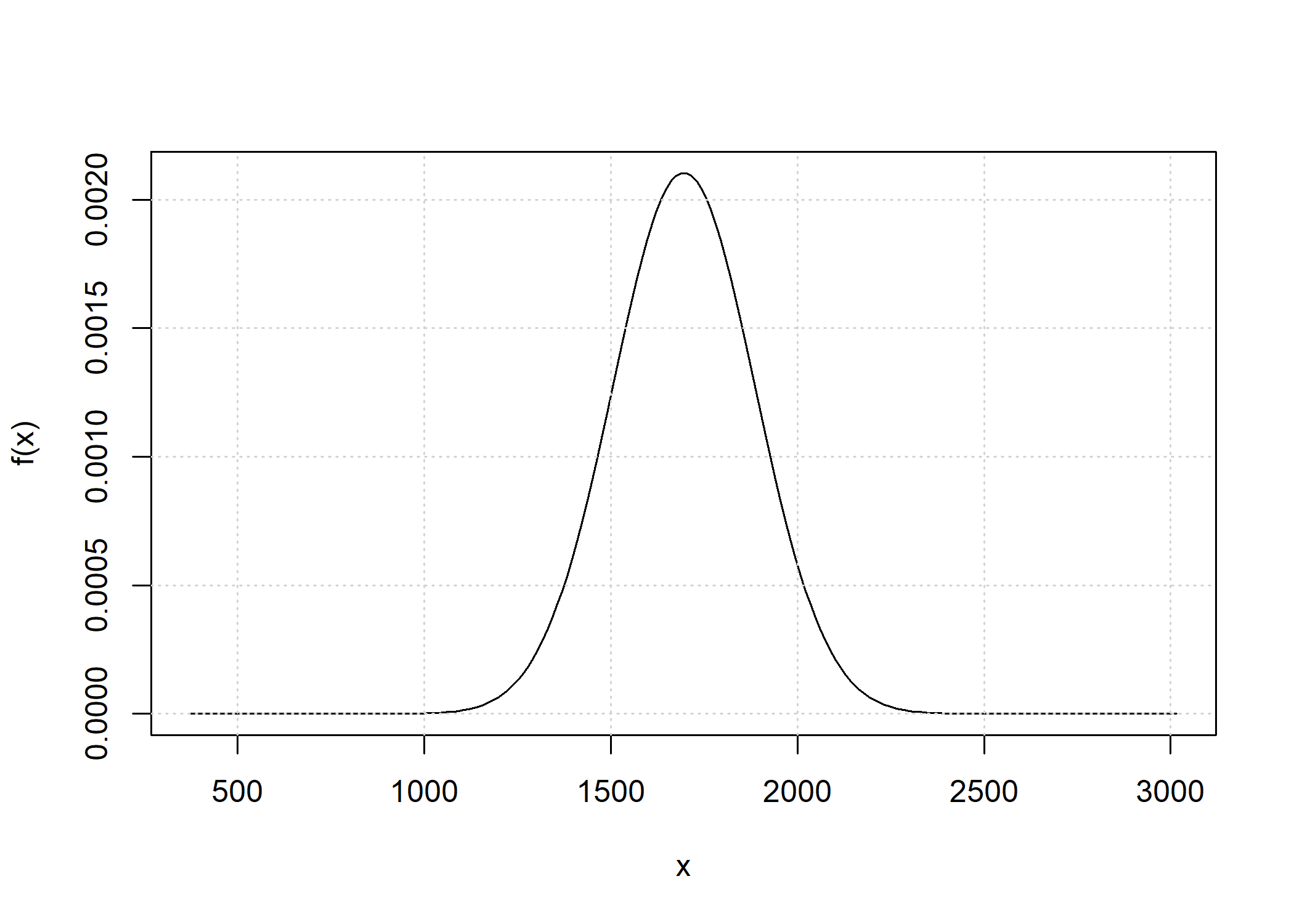
#> 1     75.16192             2

Total IBD distribution

The total_ibd_dist function obtains the full distribution of the total length of IBD segments across a chromosome. For example, we may obtain this distribution for half siblings on a chromosome with a length of 100 cM.

d_hs <- total_ibd_dist(ped_hs, chromosome_length = 100)
d_hs
#> Probability distribution of total length of segments in ibd state 1  
#> Chromosome length: 100 cM
#> 
#> Weight of continuous density: 0.8646647 
#> 
#> Point masses: 
#>    x         px
#>    0 0.06766764
#>  100 0.06766764

The distribution has two point masses (no IBD at all and fully IBD) and admits a density function otherwise. A plot includes both components.

plot(d_hs)

Utility functions for computing the expectation, variance and standard deviation of the distributions are also available. These functions use numerical integration.

E(d_hs)
#> [1] 50
sd(d_hs)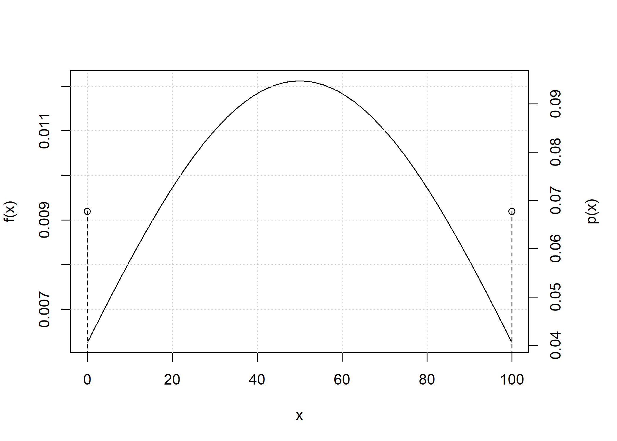
#> [1] 30.71195

Convolution of total IBD distributions

The convolution of the total IBD distribution across chromosomes is obtained when the chromosome_length parameter has length greater than 1.

d_hs_conv <- total_ibd_dist(ped_hs, 
                            chromosome_length = c(250, 200, 150, 150, 100))
plot(d_hs_conv)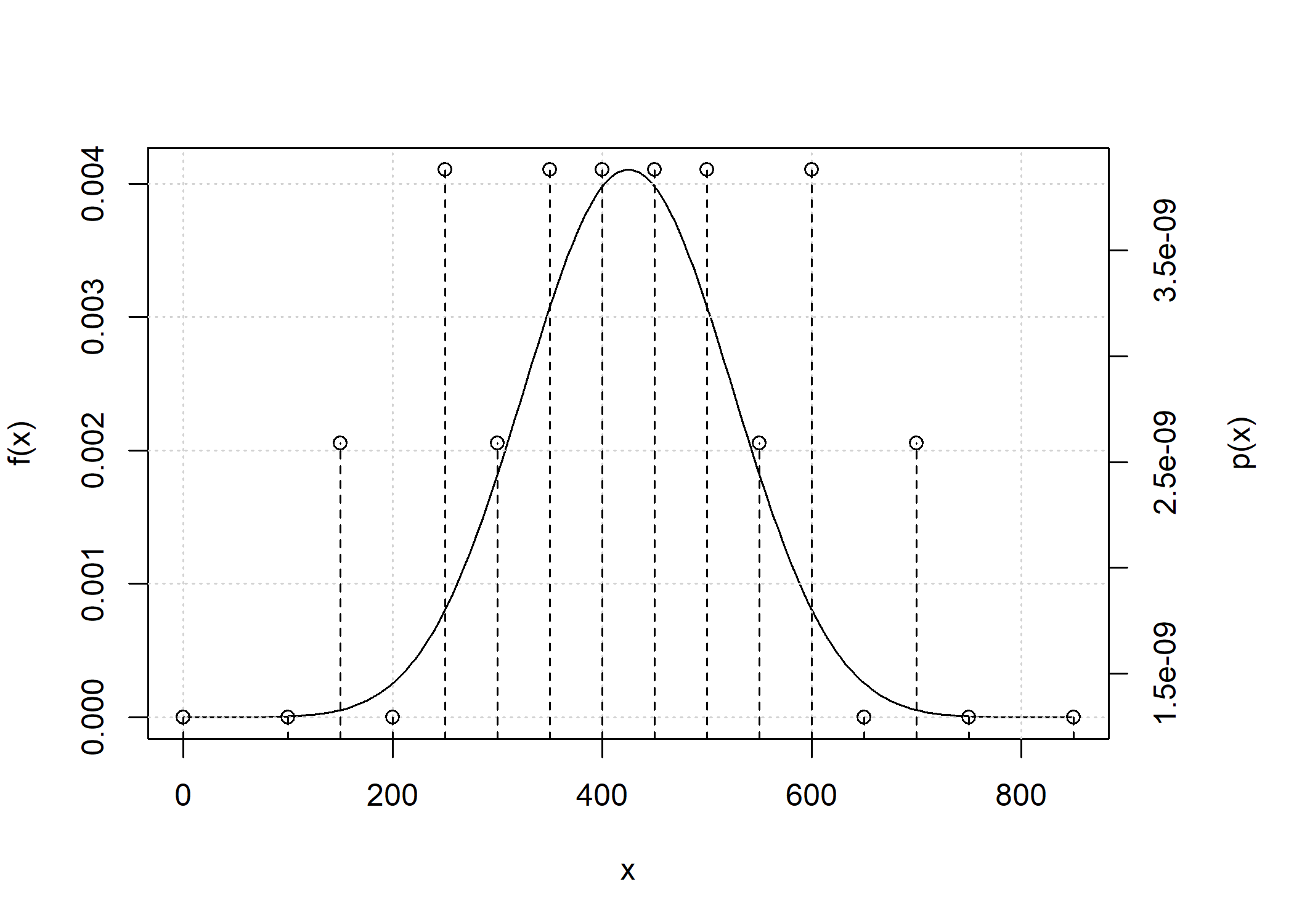

Because the number of point masses may increase quickly, by default any point mass below 1e-9 is removed.