| Type: | Package |
| Title: | Interactive Statistical Data Visualization |
| Version: | 1.4.3 |
| Date: | 2025-06-18 |
| URL: | https://great-northern-diver.github.io/loon/ |
| Description: | An extendable toolkit for interactive data visualization and exploration. |
| License: | GPL-2 |
| Depends: | R (≥ 3.5.0), methods, tcltk |
| Imports: | tools, graphics, grDevices, utils, stats, gridExtra |
| Suggests: | maps, sp, graph, scagnostics, PairViz, RColorBrewer, loon.data, rworldmap, mgcv, rgl, Rgraphviz, RDRToolbox, kernlab, scales, MASS, testthat, knitr, rmarkdown, png, formatR, covr |
| BugReports: | https://github.com/great-northern-diver/loon/issues |
| Encoding: | UTF-8 |
| LazyData: | true |
| RoxygenNote: | 7.3.2 |
| VignetteBuilder: | knitr |
| NeedsCompilation: | no |
| Packaged: | 2025-06-19 16:50:43 UTC; rwoldford |
| Author: | Adrian Waddell [aut], R. Wayne Oldford [aut, cre, ths], Zehao Xu [ctb], Martin Gauch [ctb] |
| Maintainer: | R. Wayne Oldford <rwoldford@uwaterloo.ca> |
| Repository: | CRAN |
| Date/Publication: | 2025-06-19 18:30:08 UTC |
loon: A Toolkit for Interactive Data Visualization and Exploration
Description
Loon is a toolkit for highly interactive data visualization. Interactions with plots are provided with mouse and keyboard gestures as well as via command line control and with inspectors that provide graphical user interfaces (GUIs) for modifying and overseeing plots.
Details
Currently, loon implements the following statistical graphs: histogram, scatterplot, serialaxes plot (star glyphs, parallel coordinates) and a graph display for creating navigation graphs.
Some of the implemented scatterplot features, for example, are zooming, panning, selection and moving of points, dynamic linking of plots, layering of visual information such as maps and regression lines, custom point glyphs (images, text, star glyphs), and event bindings. Event bindings provide hooks to evaluate custom code at specific plot state changes or mouse and keyboard interactions. Hence, event bindings can be used to add to or modify the default behavior of the plot widgets.
Loon's capabilities are very useful for statistical analysis tasks such as interactive exploratory data analysis, sensitivity analysis, animation, teaching, and creating new graphical user interfaces.
To get started using loon read the package vignettes or visit the loon website at https://great-northern-diver.github.io/loon/.
Author(s)
Maintainer: R. Wayne Oldford rwoldford@uwaterloo.ca [thesis advisor]
Authors:
Adrian Waddell adrian@waddell.ch
Other contributors:
Zehao Xu z267xu@uwaterloo.ca [contributor]
Martin Gauch martin.gauch@student.kit.edu [contributor]
See Also
Useful links:
Report bugs at https://github.com/great-northern-diver/loon/issues
Euclidean distance between two vectors, or between column vectors of two matrices.
Description
Quickly calculates and returns the Euclidean distances between m vectors in one set and n vectors in another. Each set of vectors is given as the columns of a matrix.
Usage
L2_distance(a, b, df = 0)
Arguments
a |
A d by m numeric matrix giving the first set of m vectors of dimension d
as the columns of |
b |
A d by n numeric matrix giving the second set of n vectors of dimension d
as the columns of |
df |
Indicator whether to force the diagonals of the returned matrix to
be zero ( |
Details
This fully vectorized (VERY FAST!) function computes the Euclidean distance between two vectors by:
||A-B|| = sqrt ( ||A||^2 + ||B||^2 - 2*A.B )
Originally written as L2_distance.m for Matlab by Roland Bunschoten of the University of Amsterdam, Netherlands.
Value
An m by n matrix containing the Euclidean distances between the column
vectors of the matrix a and the column vectors of the matrix b.
Author(s)
Roland Bunschoten (original), Adrian Waddell, Wayne Oldford
See Also
Examples
A <- matrix(rnorm(400), nrow = 10)
B <- matrix(rnorm(800), nrow = 10)
L2_distance(A[,1, drop = FALSE], B[,1, drop = FALSE])
d_AB <- L2_distance(A,B)
d_BB <- L2_distance(B,B, df = 1) # force diagonal to be zero
Data to re-create Hans Rosling's famous "Us and Them" animation
Description
This data was sourced from https://www.gapminder.org/ and contains Population, Life Expectancy, Fertility, Income, and Geographic.Region information between 1962 and 2013 for 198 countries.
Usage
UsAndThem
Format
A data frame with 9855 rows and 8 variables
- Country
country name
- Year
year of recorded measurements
- Population
country's population
- LifeExpectancy
average life expectancy in years at birth
- Fertility
in number of babies per woman
- Income
Gross domestic product per person adjusted for inflation and purchasing power (in international dollars)
- Geographic.Region
one of six large global regions
- Geographic.Region.ID
two letter identification of country
Source
Convert a loongraph object to an object of class graph
Description
Loon's native graph class is fairly basic. The graph package (on bioconductor) provides a more powerful alternative to create and work with graphs. Also, many other graph theoretic algorithms such as the complement function and some graph layout and visualization methods are implemented for the graph objects in the RBGL and Rgraphviz R packages. For more information on packages that are useful to work with graphs see the gRaphical Models in R CRAN Task View at https://cran.r-project.org/web/views/.
Usage
as.graph(loongraph)
Arguments
loongraph |
object of class loongraph |
Details
See https://www.bioconductor.org/packages/release/bioc/html/graph.html for more information about the graph R package.
Value
graph object of class loongraph
Examples
if (requireNamespace("graph", quietly = TRUE)) {
  g <- loongraph(letters[1:4], letters[1:3], letters[2:4], FALSE)
  g1 <- as.graph(g)
}
Convert a graph object to a loongraph object
Description
Sometimes it is simpler to work with objects of class loongraph than to work with object of class graph.
Usage
as.loongraph(graph)
Arguments
graph |
object of class graph (defined in the graph library) |
Details
See https://www.bioconductor.org/packages/release/bioc/html/graph.html for more information about the graph R package.
For more information run: l_help("learn_R_display_graph.html.html#graph-utilities")
Value
graph object of class loongraph
Examples
if (requireNamespace("graph", quietly = TRUE)) {
  graph_graph  = graph::randomEGraph(LETTERS[1:15], edges=100)
  loon_graph <- as.loongraph(graph_graph)
}
Turn a loon size to a grid size
Description
The size of loon is determined by pixel (px), while, in
grid graphics, the size is determined by pointsize (pt)
Usage
as_grid_size(
  size,
  type = c("points", "texts", "images", "radial", "parallel", "polygon", "lines"),
  adjust = 1,
  ...
)
Arguments
size |
input |
type |
glyph type; one of "points", "texts", "images", "radial", "parallel", "polygon", "lines". |
adjust |
a pixel (px) at 96 |
... |
some arguments used to specify the size, e.g. |
Return a 6 hexidecimal digit color representations
Description
Return a 6 hexidecimal digit color representations
Usage
as_hex6color(color)
Arguments
color |
input color |
Details
Compared with hex12tohex6(), it could accommodate 6 digit code, 12 digit code or
real color names.
See Also
l_hexcolor, hex12tohex6,
l_colorName
Examples
color <- c("#FF00FF", "#999999999999", "red")
# return 12 hexidecimal digit color
loon:::l_hexcolor(color)
# return 6 hexidecimal digit color
as_hex6color(color)
# return color names
l_colorName(color)

## Not run: # WRONG COLORS
hex12tohex6(color)
## End(Not run)
A Character Data Frame to a Numerical Data Frame
Description
Turn a data frame of characters to a data frame of numerical values. If the character cannot be converted to numerical in direct, it will be turned to factor first, then to numerical data
Usage
char2num.data.frame(chardataframe)
Arguments
chardataframe |
A char data frame |
Examples
data <- data.frame(x = c("1", "2", "3"),
                   y = c("foo", "bar", "foo"),
                   z = 4:6)
# ERROR
# data + 1
numData <- char2num.data.frame(data)
numData + 1

if(interactive()) {
  s <- l_serialaxes(iris)
  data <- s["data"]
  # it is a character data frame
  data[1,1]
  numData <- char2num.data.frame(data)
  numData[1,1]
}
Create a palette with loon's color mapping
Description
Used to map nominal data to colors. By default these colors are chosen so that the categories can be well differentiated visually (e.g. to highlight the different groups)
Usage
color_loon()
Details
This is the function that loon uses by default to map values to colors. Loon's mapping algorithm is as follows:
if all values already represent valid Tk colors (see
tkcolors) then those colors are takenif the number of distinct values is less than the number of values in loon's color mapping list then they get mapped according to the color list, see
l_setColorListandl_getColorList.if there are more distinct values than there are colors in loon's color mapping list then loon's own color mapping algorithm is used. See
loon_paletteand the details section in the documentation ofl_setColorList.
For other mappings see the col_numeric and
col_factor functions from the scales package.
Value
A function that takes a vector with values and maps them to a vector of 6 digit hexadecimal encoded color representation (strings). Note that loon uses internally 12 digit hexadecimal encoded color values. If all the values that get passed to the function are valid color names in Tcl then those colors get returned hexencoded. Otherwise, if there is one or more elements that is not a valid color name it uses the loons default color mapping algorithm.
See Also
l_setColorList, l_getColorList,
loon_palette, l_hexcolor, l_colorName,
as_hex6color
Examples
pal <- color_loon()
pal(letters[1:4])
pal(c('a','a','b','c'))
pal(c('green', 'yellow'))

# show color choices for different n's
if (requireNamespace("grid", quietly = TRUE)) {
  grid::grid.newpage()
  grid::pushViewport(grid::plotViewport())
  grid::grid.rect()
  n <- c(2,4,8,16, 21)
  # beyond this, colors are generated algorithmically
  # generating a warning
  grid::pushViewport(grid::dataViewport(xscale=c(0, max(n)+1),
                     yscale=c(0, length(n)+1)))
  grid::grid.yaxis(at=c(1:length(n)), label=paste("n =", n))
  for (i in rev(seq_along(n))) {
   cols <- pal(1:n[i])
   grid::grid.points(x = 1:n[i], y = rep(i, n[i]),
                     default.units = "native", pch=15,
                     gp=grid::gpar(col=cols))
  }
  grid::grid.text("note the first i colors are shared for each n",
                  y = grid::unit(1,"npc") + grid::unit(1, "line"))
}
Create the Complement Graph of a Graph
Description
Creates a complement graph of a graph
Usage
complement(x)
Arguments
x |
graph or loongraph object |
Value
graph object
Create the Complement Graph of a loon Graph
Description
Creates a complement graph of a graph
Usage
## S3 method for class 'loongraph'
complement(x)
Arguments
x |
loongraph object |
Details
This method is currently only implemented for undirected graphs.
Value
graph object of class loongraph
Create a complete graph or digraph with a set of nodes
Description
From Wikipedia: "a complete graph is a simple undirected graph in which every pair of distinct vertices is connected by a unique edge. A complete digraph is a directed graph in which every pair of distinct vertices is connected by a pair of unique edges (one in each direction
Usage
completegraph(nodes, isDirected = FALSE)
Arguments
nodes |
a character vector with node names, each element defines a node hence the elements need to be unique |
isDirected |
a boolean scalar to indicate wheter the returned object is a complete graph (undirected) or a complete digraph (directed). |
Details
Note that this function masks the completegraph function of the graph package. Hence it is a good idead to specify the package namespace with ::, i.e. loon::completegraph and graph::completegraph.
For more information run: l_help("learn_R_display_graph.html.html#graph-utilities")
Value
graph object of class loongraph
Examples
g <- loon::completegraph(letters[1:5])
Create a named grob or a template grob depending on a test
Description
Creates and returns a grid object using the function given by 'grobFun' when 'test' is 'TRUE' Otherwise a simple 'grob()' is produced with the same parameters. All grob parameters are given in '...'.
Usage
condGrob(test = TRUE, grobFun = grid::grob, name = "grob name", ...)
Arguments
test |
Either 'TRUE' or 'FALSE' to indicate whether 'grobFun' is to be used (default 'TRUE') or not. |
grobFun |
The function to be used to create the grob when 'test = TRUE' (e.g. 'textGrob', 'polygonGrob', etc.). |
name |
The name to be used for the returned grob. |
... |
The arguments to be given to the 'grobFun' (or to 'grob()' when 'test = FALSE'). |
Value
A grob as produced by either the 'grobFun' given or by 'grob()' using the remaining arguments. If 'test = FALSE' then the name is suffixed by ": 'grobFun name' arguments".
Examples
myGrob <- condGrob(test = (runif(1) > 0.5),
                   grobFun = textGrob,
                   name = "my label",
                   label = "Some random text")
myGrob
Layout as a grid
Description
Layout as a grid
Usage
facet_grid_layout(
  plots,
  subtitles,
  by = NULL,
  prop = 10,
  parent = NULL,
  title = "",
  xlabel = "",
  ylabel = "",
  labelLocation = c("top", "right"),
  byrow = FALSE,
  swapAxes = FALSE,
  labelBackground = l_getOption("facetLabelBackground"),
  labelForeground = l_getOption("foreground"),
  labelBorderwidth = 2,
  labelRelief = "ridge",
  plotWidth = 200,
  plotHeight = 200,
  sep = "*",
  maxCharInOneRow = 10,
  new.toplevel = TRUE,
  ...
)
Arguments
plots |
A list of |
subtitles |
The subtitles of the layout. It is a list and the length is equal to
the number of |
by |
an object of class "formula" (or one that can be coerced to that class): a symbolic description of the plots separated by |
prop |
The proportion of the label height and widget height |
parent |
a valid Tk parent widget path. When the parent widget is
specified (i.e. not |
title |
The title of the widget |
xlabel |
The xlabel of the widget |
ylabel |
The ylabel of the widget |
labelLocation |
Labels location.
|
byrow |
Place widget by row or by column |
swapAxes |
swap axes, |
labelBackground |
Label background color |
labelForeground |
Label foreground color |
labelBorderwidth |
Label border width |
labelRelief |
Label relief |
plotWidth |
default plot width (in pixel) |
plotHeight |
default plot height (in pixel) |
sep |
The character string to separate or combine a vector |
maxCharInOneRow |
deprecated |
new.toplevel |
determine whether the parent is a new top level. If it is not a new window, the widgets will not be packed |
... |
named arguments to modify plot states.
See |
layout separately
Description
layout separately
Usage
facet_separate_layout(
  plots,
  subtitles,
  title = "",
  xlabel = "",
  ylabel = "",
  sep = "*",
  maxCharInOneRow = 10,
  ...
)
Arguments
plots |
A list of |
subtitles |
The subtitles of the layout. It is a list and the length is equal to
the number of |
title |
The title of the widget |
xlabel |
The xlabel of the widget |
ylabel |
The ylabel of the widget |
sep |
The character string to separate or combine a vector |
maxCharInOneRow |
deprecated |
... |
named arguments to modify plot states.
See |
Layout as a wrap
Description
Layout as a wrap
Usage
facet_wrap_layout(
  plots,
  subtitles,
  prop = 10,
  parent = NULL,
  title = "",
  xlabel = "",
  ylabel = "",
  nrow = NULL,
  ncol = NULL,
  labelLocation = "top",
  byrow = TRUE,
  swapAxes = FALSE,
  labelBackground = l_getOption("facetLabelBackground"),
  labelForeground = l_getOption("foreground"),
  labelBorderwidth = 2,
  labelRelief = "ridge",
  plotWidth = 200,
  plotHeight = 200,
  sep = "*",
  maxCharInOneRow = 10,
  new.toplevel = TRUE,
  ...
)
Arguments
plots |
A list of |
subtitles |
The subtitles of the layout. It is a list and the length is equal to
the number of |
prop |
The proportion of the label height and widget height |
parent |
a valid Tk parent widget path. When the parent widget is
specified (i.e. not |
title |
The title of the widget |
xlabel |
The xlabel of the widget |
ylabel |
The ylabel of the widget |
nrow |
The number of layout rows |
ncol |
The number of layout columns |
labelLocation |
Labels location.
|
byrow |
Place widget by row or by column |
swapAxes |
swap axes, |
labelBackground |
Label background color |
labelForeground |
Label foreground color |
labelBorderwidth |
Label border width |
labelRelief |
Label relief |
plotWidth |
default plot width (in pixel) |
plotHeight |
default plot height (in pixel) |
sep |
The character string to separate or combine a vector |
maxCharInOneRow |
deprecated |
new.toplevel |
determine whether the parent is a new top level. If it is not a new window, the widgets will not be packed |
... |
named arguments to modify plot states.
See |
Return the Displayed Color
Description
Always reflect the current displayed color.
Usage
get_display_color(color, selected)
Arguments
color |
the |
selected |
the selected states |
Details
In loon, each element (i.e. point, bin, line) has a "temporary" color and
a "permanent" color. If one element is selected, the color is switched to the "temporary" color to highlight it.
If the selection state is eliminated, the "permanent" color of this element will be displayed.
Our function always gives the "temporary" displayed color.
Value
The color shown on the plot
Examples
if(interactive()) {
  p <- l_plot(1:10)
  p['selected'][c(1,3,5)] <- TRUE

  displayedColor <- get_display_color(p['color'], p['selected'])
  plot(1:10, bg = as_hex6color(displayedColor), pch = 21)
}
Creates a loon plot for each facet from an existing loon plot.
Description
A generic function used by l_facet when facetting an existing loon plot.
Usage
get_facets(widget, ...)
Arguments
widget |
the loon widget |
... |
other arguments to the function used to create
the loon plot for each facet. Depending on the plot being facetted, these
include the arguments |
Value
A list containing the named components plots, subtitles,
child = child, and new.toplevel containing the facets as plots
and other relevant information to construct the facetted plot.
See Also
Return Font Information
Description
Return Font Information
Usage
get_font_info_from_tk(tkFont)
Arguments
tkFont |
A specified tk font character, one of
|
Value
A list of font information, containing font "family", font "face" and font "size"
Examples
fontscales <- l_getOption("font-scales")
get_font_info_from_tk(fontscales)
Get Layer States
Description
Return the input widget states
Usage
get_layer_states(target, native_unit = TRUE, omit = NULL)
Arguments
target |
either an object of class loon or a vector that specifies the
widget, layer, glyph, navigator or context completely. The widget is
specified by the widget path name (e.g. |
native_unit |
return numerical vectors or |
omit |
deprecated |
Details
get layer states
Examples
if(interactive()){
p <- l_plot(x = c(0,1), y = c(0,1))
l <- l_layer_rectangle(p, x = c(0,0.5), y = c(0, 0.5))
# the coordinates are in `unit`
get_layer_states(p)
# the coordinates are numerical
get_layer_states(p, native_unit = FALSE)
# get `l_layer` state
get_layer_states(l)
}
Get the Order of the Display
Description
In loon, if points (in scatter plot) or lines
(in parallel or radial coordinate) are highlighted, the displayed order will be changed.
This function always reflects the current displayed order
Usage
get_model_display_order(widget)
Arguments
widget |
An |
Examples
if(interactive()) {
  p <- l_plot(rnorm(10))
  get_model_display_order(p)
  p['selected'][c(1,3,5,7)] <- TRUE
  # The 1st, 3rd, 5th, 7th points will be drawn afterwards
  # to make sure that they are displayed on top
  get_model_display_order(p)
}
Glyph to Pch
Description
turn a loon point glyph to an R graphics plotting 'character' (pch)
Usage
glyph_to_pch(glyph)
Arguments
glyph |
glyph type in |
Value
a pch type
Examples
glyph_to_pch(c("circle", "ocircle", "ccircle",
               "square", "osquare", "csquare",
               "triangle", "otriangle", "ctriangle",
               "diamond", "cdiamond", "odiamond",
               "foo"))
Make each space in a node apprear only once
Description
Reduce a graph to have unique node names
Usage
graphreduce(graph, separator)
Arguments
graph |
graph of class loongraph |
separator |
one character that separates the spaces in node names |
Details
Note this is a string based operation. Node names must not contain the separator character!
Value
graph object of class loongraph
Examples
G <- completegraph(nodes=LETTERS[1:4])
LG <- linegraph(G)

LLG <- linegraph(LG)

R_LLG <- graphreduce(LLG)
Create and optionally draw a grid grob from a loon widget handle
Description
Create and optionally draw a grid grob from a loon widget handle
Usage
grid.loon(target, name = NULL, gp = gpar(), draw = TRUE, vp = NULL)
Arguments
target |
either an object of class loon or a vector that specifies the
widget, layer, glyph, navigator or context completely. The widget is
specified by the widget path name (e.g. |
name |
a character identifier for the grob, or NULL. Used to find the grob on the display list and/or as a child of another grob. |
gp |
a gpar object, or NULL, typically the output from a call to the function gpar. This is basically a list of graphical parameter settings. |
draw |
a logical value indicating whether graphics output should be produced. |
vp |
a grid viewport object (or NULL). |
Value
a grid grob of the loon plot
See Also
Examples
## Not run:
library(grid)
widget <- with(iris, l_plot(Sepal.Length, Sepal.Width))
grid.loon(widget)

## End(Not run)
Convert 12 hexadecimal digit color representations to 6 hexidecimal digit color representations
Description
Tk colors must be in 6 hexadecimal format with two hexadecimal digits for each of the red, green, and blue components. Twelve hexadecimal digit colors have 4 hexadecimal digits for each. This function converts the 12 digit format to the 6 provided the color is preserved.
Usage
hex12tohex6(x)
Arguments
x |
a vector with 12 digit hexcolors |
Details
Function throws a warning if the conversion loses information. The
l_hexcolor function converts any Tcl color specification to a
12 digit hexadecimal color representation.
Examples
x <- l_hexcolor(c("red", "green", "blue", "orange"))
x
hex12tohex6(x)
Convert an R list to a nested Tcl list
Description
This is a helper function to create a nested Tcl list from an R list (i.e. a list of vectors).
Usage
l_Rlist2nestedTclList(x)
Arguments
x |
a list of vectors |
Value
a string that represents the tcl nested list
See Also
Examples
x <- list(c(1,3,4), c(4,3,2,1), c(4,3,2,5,6))
l_Rlist2nestedTclList(x)
Evaluate a function on once the processor is idle
Description
It is possible for an observer to call the configure method of that plot while the plot is still in the configuration pipeline. In this case, a warning is thrown as unwanted side effects can happen if the next observer in line gets an outdated notification. In this case, it is recommended to use the l_after_idle function that evaluates some code once the processor is idle.
Usage
l_after_idle(fun)
Arguments
fun |
function to be evaluated once tcl interpreter is idle |
Query the aspect ratio of a plot
Description
The aspect ratio is defined by the ratio of the number of pixels for one data unit on the y axis and the number of pixels for one data unit on the x axes.
Usage
l_aspect(widget)
Arguments
widget |
widget path as a string or as an object handle |
Value
aspect ratio
Examples
## Not run:
p <- with(iris, l_plot(Sepal.Length ~ Sepal.Width, color=Species))

l_aspect(p)
l_aspect(p) <- 1

## End(Not run)
Set the aspect ratio of a plot
Description
The aspect ratio is defined by the ratio of the number of pixels for one data unit on the y axis and the number of pixels for one data unit on the x axes.
Usage
l_aspect(widget) <- value
Arguments
widget |
widget path as a string or as an object handle |
value |
aspect ratio |
Details
Changing the aspect ratio with l_aspect<- changes effectively
the zoomY state to obtain the desired aspect ratio. Note that the
aspect ratio in loon depends on the plot width, plot height and the states
zoomX, zoomY, deltaX, deltaY and
swapAxes. Hence, the aspect aspect ratio can not be set permanently
for a loon plot.
Examples
## Not run:
p <- with(iris, l_plot(Sepal.Length ~ Sepal.Width, color=Species))

l_aspect(p)
l_aspect(p) <- 1

## End(Not run)
Get the set of basic path types for loon plots.
Description
Loon's plots are constructed in TCL and identified with a path string appearing in the window containing the plot. The path string begins with a unique identifier for the plot and ends with a suffix describing the type of loon plot being displayed.
The path identifying the plot is the string concatenation of both the identifier and the type.
This function returns the set of the base (non-compound) loon path types.
Usage
l_basePaths()
Value
character vector of the base path types.
See Also
l_compoundPaths l_getFromPath l_loonWidgets
Get labels for each observation according to bin cuts in the histogram.
Description
l_binCut divides l_hist widget x into current histogram intervals and codes values
x according to which interval they fall (if active). It is modelled on cut in base package.
Usage
l_binCut(widget, labels, digits = 2, inactive)
Arguments
widget |
A loon histogram widget. |
labels |
Labels to identify which bin observations are in.
By default, labels are constructed using "(a,b]" interval notation.
If |
digits |
The number of digits used in formatting the breaks for default labels. |
inactive |
The value to use for inactive observations when labels is a vector.
Default depends on |
Value
A vector of bin identifiers having length equal to the total number of observations in the histogram.
The type of vector depends on the labels argument.
For default labels = NULL, a factor is returned, for labels = FALSE, a vector of bin numbers, and
for arbitrary vector labels a vector of bins labelled in order of labels will be returned.
Inactive cases appear in no bin and so are assigned the value of active when given.
The default active value also depends on labels: when labels = NULL, the default active is "(-Inf, Inf)";
when labels = FALSE, the default active is -1; and when labels is a vector of length equal
to the number of bins, the default active is NA.
The value of active denotes the bin name for the inactive cases.
See Also
l_getBinData, l_getBinIds, l_breaks
Examples
if(interactive()) {
h <- l_hist(iris)
h["active"] <- iris$Species != "setosa"
binCut <- l_binCut(h)
h['color'] <- binCut
## number of bins
nBins <- length(l_getBinIds(h))
## ggplot color hue
gg_color_hue <- function(n) {
  hues <- seq(15, 375, length = n + 1)
  hcl(h = hues, l = 65, c = 100)[1:n]
}
h['color'] <- l_binCut(h, labels = gg_color_hue(nBins), inactive = "firebrick")
h["active"] <- TRUE
}
Create a Canvas Binding
Description
Canvas bindings are triggered by a mouse/keyboard gesture over the plot as a whole.
Usage
l_bind_canvas(widget, event, callback)
Arguments
widget |
widget path as a string or as an object handle |
event |
event patterns as defined for Tk canvas widget https://www.tcl-lang.org/man/tcl8.6/TkCmd/bind.htm#M5. |
callback |
callback function is an R function which is called by the Tcl interpreter if the event of interest happens. Note that in loon the callback functions support different optional arguments depending on the binding type, read the details for more information |
Details
Canvas bindings are used to evaluate callbacks at certain X events on the canvas widget (underlying widget for all of loon's plot widgets). Such X events include re-sizing of the canvas and entering the canvas with the mouse.
Bindings, callbacks, and binding substitutions are described in detail in
loon's documentation webpage, i.e. run l_help("learn_R_bind")
Value
canvas binding id
See Also
l_bind_canvas_ids, l_bind_canvas_get,
l_bind_canvas_delete, l_bind_canvas_reorder
Examples
# binding for when plot is resized
if(interactive()){
p <- l_plot(iris[,1:2], color=iris$Species)

printSize <- function(p) {
    size <- l_size(p)
    cat(paste('Size of widget ', p, ' is: ',
              size[1], 'x', size[2], ' pixels\n', sep=''))
}

l_bind_canvas(p, event='<Configure>', function(W) {printSize(W)})

id <- l_bind_canvas_ids(p)
id

l_bind_canvas_get(p, id)

}
Delete a canvas binding
Description
Remove a canvas binding
Usage
l_bind_canvas_delete(widget, id)
Arguments
widget |
widget path as a string or as an object handle |
id |
canvas binding id |
Details
Bindings, callbacks, and binding substitutions are described in detail in
loon's documentation webpage, i.e. run l_help("learn_R_bind")
See Also
l_bind_canvas, l_bind_canvas_ids,
l_bind_canvas_get, l_bind_canvas_reorder
Get the event pattern and callback Tcl code of a canvas binding
Description
This function returns the registered event pattern and the Tcl callback code that the Tcl interpreter evaluates after a event occurs that matches the event pattern.
Usage
l_bind_canvas_get(widget, id)
Arguments
widget |
widget path as a string or as an object handle |
id |
canvas binding id |
Details
Bindings, callbacks, and binding substitutions are described in detail in
loon's documentation webpage, i.e. run l_help("learn_R_bind")
Value
Character vector of length two. First element is the event pattern, the second element is the Tcl callback code.
See Also
l_bind_canvas, l_bind_canvas_ids,
l_bind_canvas_delete, l_bind_canvas_reorder
Examples
# binding for when plot is resized
if(interactive()){
p <- l_plot(iris[,1:2], color=iris$Species)

printSize <- function(p) {
    size <- l_size(p)
    cat(paste('Size of widget ', p, ' is: ',
              size[1], 'x', size[2], ' pixels\n', sep=''))
}

l_bind_canvas(p, event='<Configure>', function(W) {printSize(W)})

id <- l_bind_canvas_ids(p)
id

l_bind_canvas_get(p, id)

}
List canvas binding ids
Description
List all user added canvas binding ids
Usage
l_bind_canvas_ids(widget)
Arguments
widget |
widget path as a string or as an object handle |
Details
Bindings, callbacks, and binding substitutions are described in detail in
loon's documentation webpage, i.e. run l_help("learn_R_bind")
Value
vector with canvas binding ids
See Also
l_bind_canvas, l_bind_canvas_get,
l_bind_canvas_delete, l_bind_canvas_reorder
Examples
# binding for when plot is resized
if(interactive()){
p <- l_plot(iris[,1:2], color=iris$Species)

printSize <- function(p) {
    size <- l_size(p)
    cat(paste('Size of widget ', p, ' is: ',
              size[1], 'x', size[2], ' pixels\n', sep=''))
}

l_bind_canvas(p, event='<Configure>', function(W) {printSize(W)})

id <- l_bind_canvas_ids(p)
id

l_bind_canvas_get(p, id)

}
Reorder the canvas binding evaluation sequence
Description
The order the canvas bindings defines how they get evaluated once an event matches event patterns of multiple canvas bindings.
Usage
l_bind_canvas_reorder(widget, ids)
Arguments
widget |
widget path as a string or as an object handle |
ids |
new canvas binding id evaluation order, this must be a
rearrangement of the elements returned by the
|
Details
Bindings, callbacks, and binding substitutions are described in detail in
loon's documentation webpage, i.e. run l_help("learn_R_bind")
Value
vector with binding id evaluation order (same as the id argument)
See Also
l_bind_canvas, l_bind_canvas_ids,
l_bind_canvas_get, l_bind_canvas_delete
Add a context binding
Description
Creates a binding that evaluates a callback for particular changes in the collection of contexts of a display.
Usage
l_bind_context(widget, event, callback)
Arguments
widget |
widget path as a string or as an object handle |
event |
a vector with one or more of the following events: |
callback |
callback function is an R function which is called by the Tcl interpreter if the event of interest happens. Note that in loon the callback functions support different optional arguments depending on the binding type, read the details for more information |
Details
Bindings, callbacks, and binding substitutions are described in detail in
loon's documentation webpage, i.e. run l_help("learn_R_bind")
Value
context binding id
See Also
l_bind_context_ids, l_bind_context_get,
l_bind_context_delete, l_bind_context_reorder
Delete a context binding
Description
Remove a context binding
Usage
l_bind_context_delete(widget, id)
Arguments
widget |
widget path as a string or as an object handle |
id |
context binding id |
Details
Bindings, callbacks, and binding substitutions are described in detail in
loon's documentation webpage, i.e. run l_help("learn_R_bind")
See Also
l_bind_context, l_bind_context_ids,
l_bind_context_get, l_bind_context_reorder
Get the event pattern and callback Tcl code of a context binding
Description
This function returns the registered event pattern and the Tcl callback code that the Tcl interpreter evaluates after a event occurs that matches the event pattern.
Usage
l_bind_context_get(widget, id)
Arguments
widget |
widget path as a string or as an object handle |
id |
context binding id |
Details
Bindings, callbacks, and binding substitutions are described in detail in
loon's documentation webpage, i.e. run l_help("learn_R_bind")
Value
Character vector of length two. First element is the event pattern, the second element is the Tcl callback code.
See Also
l_bind_context, l_bind_context_ids,
l_bind_context_delete, l_bind_context_reorder
List context binding ids
Description
List all user added context binding ids
Usage
l_bind_context_ids(widget)
Arguments
widget |
widget path as a string or as an object handle |
Details
Bindings, callbacks, and binding substitutions are described in detail in
loon's documentation webpage, i.e. run l_help("learn_R_bind")
Value
vector with context binding ids
See Also
l_bind_context, l_bind_context_get,
l_bind_context_delete, l_bind_context_reorder
Reorder the context binding evaluation sequence
Description
The order the context bindings defines how they get evaluated once an event matches event patterns of multiple context bindings.
Usage
l_bind_context_reorder(widget, ids)
Arguments
widget |
widget path as a string or as an object handle |
ids |
new context binding id evaluation order, this must be a
rearrangement of the elements returned by the
|
Details
Bindings, callbacks, and binding substitutions are described in detail in
loon's documentation webpage, i.e. run l_help("learn_R_bind")
Value
vector with binding id evaluation order (same as the id argument)
See Also
l_bind_context, l_bind_context_ids,
l_bind_context_get, l_bind_context_delete
Add a glyph binding
Description
Creates a binding that evaluates a callback for particular changes in the collection of glyphs of a display.
Usage
l_bind_glyph(widget, event, callback)
Arguments
widget |
widget path as a string or as an object handle |
event |
a vector with one or more of the following events: |
callback |
callback function is an R function which is called by the Tcl interpreter if the event of interest happens. Note that in loon the callback functions support different optional arguments depending on the binding type, read the details for more information |
Details
Bindings, callbacks, and binding substitutions are described in detail in
loon's documentation webpage, i.e. run l_help("learn_R_bind")
Value
glyph binding id
See Also
l_bind_glyph_ids, l_bind_glyph_get,
l_bind_glyph_delete, l_bind_glyph_reorder
Delete a glyph binding
Description
Remove a glyph binding
Usage
l_bind_glyph_delete(widget, id)
Arguments
widget |
widget path as a string or as an object handle |
id |
glyph binding id |
Details
Bindings, callbacks, and binding substitutions are described in detail in
loon's documentation webpage, i.e. run l_help("learn_R_bind")
See Also
l_bind_glyph, l_bind_glyph_ids,
l_bind_glyph_get, l_bind_glyph_reorder
Get the event pattern and callback Tcl code of a glyph binding
Description
This function returns the registered event pattern and the Tcl callback code that the Tcl interpreter evaluates after a event occurs that matches the event pattern.
Usage
l_bind_glyph_get(widget, id)
Arguments
widget |
widget path as a string or as an object handle |
id |
glyph binding id |
Details
Bindings, callbacks, and binding substitutions are described in detail in
loon's documentation webpage, i.e. run l_help("learn_R_bind")
Value
Character vector of length two. First element is the event pattern, the second element is the Tcl callback code.
See Also
l_bind_glyph, l_bind_glyph_ids,
l_bind_glyph_delete, l_bind_glyph_reorder
List glyph binding ids
Description
List all user added glyph binding ids
Usage
l_bind_glyph_ids(widget)
Arguments
widget |
widget path as a string or as an object handle |
Details
Bindings, callbacks, and binding substitutions are described in detail in
loon's documentation webpage, i.e. run l_help("learn_R_bind")
Value
vector with glyph binding ids
See Also
l_bind_glyph, l_bind_glyph_get,
l_bind_glyph_delete, l_bind_glyph_reorder
Reorder the glyph binding evaluation sequence
Description
The order the glyph bindings defines how they get evaluated once an event matches event patterns of multiple glyph bindings.
Usage
l_bind_glyph_reorder(widget, ids)
Arguments
widget |
widget path as a string or as an object handle |
ids |
new glyph binding id evaluation order, this must be a
rearrangement of the elements returned by the
|
Details
Bindings, callbacks, and binding substitutions are described in detail in
loon's documentation webpage, i.e. run l_help("learn_R_bind")
Value
vector with binding id evaluation order (same as the id argument)
See Also
l_bind_glyph, l_bind_glyph_ids,
l_bind_glyph_get, l_bind_glyph_delete
Create a Canvas Binding
Description
Canvas bindings are triggered by a mouse/keyboard gesture over the plot as a whole.
Usage
l_bind_item(widget, tags, event, callback)
Arguments
widget |
widget path as a string or as an object handle |
tags |
item tags as as explained in
|
event |
event patterns as defined for Tk canvas widget https://www.tcl-lang.org/man/tcl8.6/TkCmd/bind.htm#M5. |
callback |
callback function is an R function which is called by the Tcl interpreter if the event of interest happens. Note that in loon the callback functions support different optional arguments depending on the binding type, read the details for more information |
Details
Item bindings are used for evaluating callbacks at certain mouse and/or keyboard gestures events (i.e. X events) on visual items on the canvas. Items on the canvas can have tags and item bindings are specified to be evaluated at certain X events for items with specific tags.
Note that item bindings get currently evaluated in the order that they are added.
Bindings, callbacks, and binding substitutions are described in detail in
loon's documentation webpage, i.e. run l_help("learn_R_bind")
Value
item binding id
See Also
l_bind_item_ids, l_bind_item_get,
l_bind_item_delete, l_bind_item_reorder
Delete a item binding
Description
Remove a item binding
Usage
l_bind_item_delete(widget, id)
Arguments
widget |
widget path as a string or as an object handle |
id |
item binding id |
Details
Bindings, callbacks, and binding substitutions are described in detail in
loon's documentation webpage, i.e. run l_help("learn_R_bind")
See Also
l_bind_item, l_bind_item_ids,
l_bind_item_get, l_bind_item_reorder
Get the event pattern and callback Tcl code of a item binding
Description
This function returns the registered event pattern and the Tcl callback code that the Tcl interpreter evaluates after a event occurs that matches the event pattern.
Usage
l_bind_item_get(widget, id)
Arguments
widget |
widget path as a string or as an object handle |
id |
item binding id |
Details
Bindings, callbacks, and binding substitutions are described in detail in
loon's documentation webpage, i.e. run l_help("learn_R_bind")
Value
Character vector of length two. First element is the event pattern, the second element is the Tcl callback code.
See Also
l_bind_item, l_bind_item_ids,
l_bind_item_delete, l_bind_item_reorder
List item binding ids
Description
List all user added item binding ids
Usage
l_bind_item_ids(widget)
Arguments
widget |
widget path as a string or as an object handle |
Details
Bindings, callbacks, and binding substitutions are described in detail in
loon's documentation webpage, i.e. run l_help("learn_R_bind")
Value
vector with item binding ids
See Also
l_bind_item, l_bind_item_get,
l_bind_item_delete, l_bind_item_reorder
Reorder the item binding evaluation sequence
Description
The order the item bindings defines how they get evaluated once an event matches event patterns of multiple item bindings.
Reordering item bindings has currently no effect. Item bindings are evaluated in the order in which they have been added.
Usage
l_bind_item_reorder(widget, ids)
Arguments
widget |
widget path as a string or as an object handle |
ids |
new item binding id evaluation order, this must be a
rearrangement of the elements returned by the
|
Details
Bindings, callbacks, and binding substitutions are described in detail in
loon's documentation webpage, i.e. run l_help("learn_R_bind")
Value
vector with binding id evaluation order (same as the id argument)
See Also
l_bind_item, l_bind_item_ids,
l_bind_item_get, l_bind_item_delete
Add a layer binding
Description
Creates a binding that evaluates a callback for particular changes in the collection of layers of a display.
Usage
l_bind_layer(widget, event, callback)
Arguments
widget |
widget path as a string or as an object handle |
event |
a vector with one or more of the following events: |
callback |
callback function is an R function which is called by the Tcl interpreter if the event of interest happens. Note that in loon the callback functions support different optional arguments depending on the binding type, read the details for more information |
Details
Bindings, callbacks, and binding substitutions are described in detail in
loon's documentation webpage, i.e. run l_help("learn_R_bind")
Value
layer binding id
See Also
l_bind_layer_ids, l_bind_layer_get,
l_bind_layer_delete, l_bind_layer_reorder
Delete a layer binding
Description
Remove a layer binding
Usage
l_bind_layer_delete(widget, id)
Arguments
widget |
widget path as a string or as an object handle |
id |
layer binding id |
Details
Bindings, callbacks, and binding substitutions are described in detail in
loon's documentation webpage, i.e. run l_help("learn_R_bind")
See Also
l_bind_layer, l_bind_layer_ids,
l_bind_layer_get, l_bind_layer_reorder
Get the event pattern and callback Tcl code of a layer binding
Description
This function returns the registered event pattern and the Tcl callback code that the Tcl interpreter evaluates after a event occurs that matches the event pattern.
Usage
l_bind_layer_get(widget, id)
Arguments
widget |
widget path as a string or as an object handle |
id |
layer binding id |
Details
Bindings, callbacks, and binding substitutions are described in detail in
loon's documentation webpage, i.e. run l_help("learn_R_bind")
Value
Character vector of length two. First element is the event pattern, the second element is the Tcl callback code.
See Also
l_bind_layer, l_bind_layer_ids,
l_bind_layer_delete, l_bind_layer_reorder
List layer binding ids
Description
List all user added layer binding ids
Usage
l_bind_layer_ids(widget)
Arguments
widget |
widget path as a string or as an object handle |
Details
Bindings, callbacks, and binding substitutions are described in detail in
loon's documentation webpage, i.e. run l_help("learn_R_bind")
Value
vector with layer binding ids
See Also
l_bind_layer, l_bind_layer_get,
l_bind_layer_delete, l_bind_layer_reorder
Reorder the layer binding evaluation sequence
Description
The order the layer bindings defines how they get evaluated once an event matches event patterns of multiple layer bindings.
Usage
l_bind_layer_reorder(widget, ids)
Arguments
widget |
widget path as a string or as an object handle |
ids |
new layer binding id evaluation order, this must be a
rearrangement of the elements returned by the
|
Details
Bindings, callbacks, and binding substitutions are described in detail in
loon's documentation webpage, i.e. run l_help("learn_R_bind")
Value
vector with binding id evaluation order (same as the id argument)
See Also
l_bind_layer, l_bind_layer_ids,
l_bind_layer_get, l_bind_layer_delete
Add a navigator binding
Description
Creates a binding that evaluates a callback for particular changes in the collection of navigators of a display.
Usage
l_bind_navigator(widget, event, callback)
Arguments
widget |
widget path as a string or as an object handle |
event |
a vector with one or more of the following events: |
callback |
callback function is an R function which is called by the Tcl interpreter if the event of interest happens. Note that in loon the callback functions support different optional arguments depending on the binding type, read the details for more information |
Details
Bindings, callbacks, and binding substitutions are described in detail in
loon's documentation webpage, i.e. run l_help("learn_R_bind")
Value
navigator binding id
See Also
l_bind_navigator_ids, l_bind_navigator_get,
l_bind_navigator_delete, l_bind_navigator_reorder
Delete a navigator binding
Description
Remove a navigator binding
Usage
l_bind_navigator_delete(widget, id)
Arguments
widget |
widget path as a string or as an object handle |
id |
navigator binding id |
Details
Bindings, callbacks, and binding substitutions are described in detail in
loon's documentation webpage, i.e. run l_help("learn_R_bind")
See Also
l_bind_navigator, l_bind_navigator_ids,
l_bind_navigator_get, l_bind_navigator_reorder
Get the event pattern and callback Tcl code of a navigator binding
Description
This function returns the registered event pattern and the Tcl callback code that the Tcl interpreter evaluates after a event occurs that matches the event pattern.
Usage
l_bind_navigator_get(widget, id)
Arguments
widget |
widget path as a string or as an object handle |
id |
navigator binding id |
Details
Bindings, callbacks, and binding substitutions are described in detail in
loon's documentation webpage, i.e. run l_help("learn_R_bind")
Value
Character vector of length two. First element is the event pattern, the second element is the Tcl callback code.
See Also
l_bind_navigator, l_bind_navigator_ids,
l_bind_navigator_delete, l_bind_navigator_reorder
List navigator binding ids
Description
List all user added navigator binding ids
Usage
l_bind_navigator_ids(widget)
Arguments
widget |
widget path as a string or as an object handle |
Details
Bindings, callbacks, and binding substitutions are described in detail in
loon's documentation webpage, i.e. run l_help("learn_R_bind")
Value
vector with navigator binding ids
See Also
l_bind_navigator, l_bind_navigator_get,
l_bind_navigator_delete, l_bind_navigator_reorder
Reorder the navigator binding evaluation sequence
Description
The order the navigator bindings defines how they get evaluated once an event matches event patterns of multiple navigator bindings.
Usage
l_bind_navigator_reorder(widget, ids)
Arguments
widget |
widget path as a string or as an object handle |
ids |
new navigator binding id evaluation order, this must be a
rearrangement of the elements returned by the
|
Details
Bindings, callbacks, and binding substitutions are described in detail in
loon's documentation webpage, i.e. run l_help("learn_R_bind")
Value
vector with binding id evaluation order (same as the id argument)
See Also
l_bind_navigator, l_bind_navigator_ids,
l_bind_navigator_get, l_bind_navigator_delete
Add a state change binding
Description
The callback of a state change binding is evaluated when certain states change, as specified at binding creation.
Usage
l_bind_state(target, event, callback)
Arguments
target |
either an object of class loon or a vector that specifies the
widget, layer, glyph, navigator or context completely. The widget is
specified by the widget path name (e.g. |
event |
vector with state names |
callback |
callback function is an R function which is called by the Tcl interpreter if the event of interest happens. Note that in loon the callback functions support different optional arguments depending on the binding type, read the details for more information |
Details
Bindings, callbacks, and binding substitutions are described in detail in
loon's documentation webpage, i.e. run l_help("learn_R_bind")
Value
state change binding id
See Also
l_info_states, l_bind_state_ids,
l_bind_state_get, l_bind_state_delete,
l_bind_state_reorder
Delete a state binding
Description
Remove a state binding
Usage
l_bind_state_delete(target, id)
Arguments
target |
either an object of class loon or a vector that specifies the
widget, layer, glyph, navigator or context completely. The widget is
specified by the widget path name (e.g. |
id |
state binding id |
Details
Bindings, callbacks, and binding substitutions are described in detail in
loon's documentation webpage, i.e. run l_help("learn_R_bind")
See Also
l_bind_state, l_bind_state_ids,
l_bind_state_get, l_bind_state_reorder
Get the event pattern and callback Tcl code of a state binding
Description
This function returns the registered event pattern and the Tcl callback code that the Tcl interpreter evaluates after a event occurs that matches the event pattern.
Usage
l_bind_state_get(target, id)
Arguments
target |
either an object of class loon or a vector that specifies the
widget, layer, glyph, navigator or context completely. The widget is
specified by the widget path name (e.g. |
id |
state binding id |
Details
Bindings, callbacks, and binding substitutions are described in detail in
loon's documentation webpage, i.e. run l_help("learn_R_bind")
Value
Character vector of length two. First element is the event pattern, the second element is the Tcl callback code.
See Also
l_bind_state, l_bind_state_ids,
l_bind_state_delete, l_bind_state_reorder
List state binding ids
Description
List all user added state binding ids
Usage
l_bind_state_ids(target)
Arguments
target |
either an object of class loon or a vector that specifies the
widget, layer, glyph, navigator or context completely. The widget is
specified by the widget path name (e.g. |
Details
Bindings, callbacks, and binding substitutions are described in detail in
loon's documentation webpage, i.e. run l_help("learn_R_bind")
Value
vector with state binding ids
See Also
l_bind_state, l_bind_state_get,
l_bind_state_delete, l_bind_state_reorder
Reorder the state binding evaluation sequence
Description
The order the state bindings defines how they get evaluated once an event matches event patterns of multiple state bindings.
Usage
l_bind_state_reorder(target, ids)
Arguments
target |
either an object of class loon or a vector that specifies the
widget, layer, glyph, navigator or context completely. The widget is
specified by the widget path name (e.g. |
ids |
new state binding id evaluation order, this must be a
rearrangement of the elements returned by the
|
Details
Bindings, callbacks, and binding substitutions are described in detail in
loon's documentation webpage, i.e. run l_help("learn_R_bind")
Value
vector with binding id evaluation order (same as the id argument)
See Also
l_bind_state, l_bind_state_ids,
l_bind_state_get, l_bind_state_delete
Gets the boundaries of the histogram bins containing active points.
Description
Queries the histogram and returns the ids of all active points in each bin that contains active points.
Usage
l_breaks(widget)
Arguments
widget |
A loon histogram widget. |
Value
A named list of the minimum and maximum values of the boundaries for each active bins in the histogram.
See Also
l_getBinData, l_getBinIds,
l_binCut
Query a Plot State
Description
All of loon's displays have plot states. Plot states specify what is displayed, how it is displayed and if and how the plot is linked with other loon plots. Layers, glyphs, navigators and contexts have states too (also refered to as plot states). This function queries a single plot state.
Usage
l_cget(target, state)
Arguments
target |
either an object of class loon or a vector that specifies the
widget, layer, glyph, navigator or context completely. The widget is
specified by the widget path name (e.g. |
state |
state name |
See Also
l_configure, l_info_states,
l_create_handle
Examples
if(interactive()){

p <- l_plot(iris, color = iris$Species)
l_cget(p, "color")
p['selected']
}
Convert color representations having an alpha transparency level to 6 digit color representations
Description
Colors in the standard tk used by loon do not allow for alpha transparency.
This function allows loon to use color palettes (e.g. l_setColorList) that
produce colors with alpha transparency by simply using only the rgb.
Usage
l_colRemoveAlpha(col)
Arguments
col |
a vector of colors (potentially) containing an alpha level |
Examples
x <- l_colRemoveAlpha(rainbow(6))
# Also works with ordinary color string representations
# since it just extracts the rgb values from the colors.
x <- l_colRemoveAlpha(c("red", "blue", "green", "orange"))
x
Get Color Names from the Hex Code
Description
Return the built-in color names by the given hex code.
Usage
l_colorName(color, error = TRUE, precise = FALSE)
Arguments
color |
A vector of 12 digit (tcl) or 6 (8 with transparency) digit color hex code, e.g. "#FFFF00000000", "#FF0000" |
error |
Suppose the input is not a valid color, if |
precise |
Logical; When |
Details
Function colors returns the built-in color names
which R knows about. To convert a hex code to a real color name,
we first convert these built-in colours and the hex code to RGB (red/green/blue) values
(e.g., "black" –> [0, 0, 0]). Then, using this RGB vector value,
the closest (Euclidean distance) built-in colour is determined.
Matching is "precise" whenever the minimum distance is zero;
otherwise it is "approximate",
locating the nearest R colour.
Value
A vector of built-in color names
See Also
l_hexcolor, hex12tohex6,
as_hex6color
Examples
l_colorName(c("#FFFF00000000", "#FF00FF", "blue"))

if(require(grid)) {
# redGradient is a matrix of 20 different colors
redGradient <- matrix(hcl(0, 80, seq(49, 68, 1)),
                      nrow=4, ncol=5, byrow = TRUE)
# a color plate
grid::grid.newpage()
grid::grid.raster(redGradient,
                  interpolate = FALSE)

# a "rough matching";
r <- l_colorName(redGradient)
# the color name of each row is identical...
r
grid::grid.newpage()
# very different from the first plate
grid::grid.raster(r, interpolate = FALSE)

# a "precise matching";
p <- l_colorName(redGradient, precise = TRUE)
# no built-in color names can be precisely matched...
p
}
## Not run:
# an error will be returned
l_colorName(c("foo", "bar", "red"))

# c("foo", "bar", "red") will be returned
l_colorName(c("foo", "bar", "#FFFF00000000"), error = FALSE)

## End(Not run)
Get the set of basic path types for loon plots.
Description
Loon's plots are constructed in TCL and identified with a path string appearing in the window containing the plot. The path string begins with a unique identifier for the plot and ends with a suffix describing the type of loon plot being displayed.
The path identifying the plot is the string concatenation of both the identifier and the type.
This function returns the set of the loon path types for compound loon plots.
Usage
l_compoundPaths()
Value
character vector of the compound path types.
See Also
l_basePathsl_loonWidgets l_getFromPath
Modify one or multiple plot states
Description
All of loon's displays have plot states. Plot states specify what is displayed, how it is displayed and if and how the plot is linked with other loon plots. Layers, glyphs, navigators and contexts have states too (also refered to as plot states). This function modifies one or multiple plot states.
Usage
l_configure(target, ...)
Arguments
target |
either an object of class loon or a vector that specifies the
widget, layer, glyph, navigator or context completely. The widget is
specified by the widget path name (e.g. |
... |
state=value pairs |
See Also
l_cget, l_info_states,
l_create_handle
Examples
if(interactive()){

p <- l_plot(iris, color = iris$Species)
l_configure(p, color='red')
p['size'] <- ifelse(iris$Species == "versicolor", 2, 8)
}
Create a context2d navigator context
Description
A context2d maps every location on a 2d space graph to a list of xvars and a list of yvars such that, while moving the navigator along the graph, as few changes as possible take place in xvars and yvars.
Contexts are in more detail explained in the webmanual accessible with
l_help. Please read the section on context by running
l_help("learn_R_display_graph.html#contexts").
Usage
l_context_add_context2d(navigator, ...)
Arguments
navigator |
navigator handle object |
... |
arguments passed on to modify context states |
Value
context handle
See Also
l_info_states, l_context_ids,
l_context_add_geodesic2d,
l_context_add_slicing2d, l_context_getLabel,
l_context_relabel
Create a geodesic2d navigator context
Description
Geodesic2d maps every location on the graph as an orthogonal projection of the data onto a two-dimensional subspace. The nodes then represent the sub-space spanned by a pair of variates and the edges either a 3d- or 4d-transition of one scatterplot into another, depending on how many variates the two nodes connected by the edge share (see Hurley and Oldford 2011). The geodesic2d context inherits from the context2d context.
Contexts are in more detail explained in the webmanual accessible with
l_help. Please read the section on context by running
l_help("learn_R_display_graph.html#contexts").
Usage
l_context_add_geodesic2d(navigator, ...)
Arguments
navigator |
navigator handle object |
... |
arguments passed on to modify context states |
Value
context handle
See Also
l_info_states, l_context_ids,
l_context_add_context2d,
l_context_add_slicing2d, l_context_getLabel,
l_context_relabel
Create a slicind2d navigator context
Description
The slicing2d context implements slicing using navigation graphs and a scatterplot to condition on one or two variables.
Contexts are in more detail explained in the webmanual accessible with
l_help. Please read the section on context by running
l_help("learn_R_display_graph.html#contexts").
Usage
l_context_add_slicing2d(navigator, ...)
Arguments
navigator |
navigator handle object |
... |
arguments passed on to modify context states |
Value
context handle
Examples
if(interactive()){

names(oliveAcids) <- c('p','p1','s','o','l','l1','a','e')
nodes <- apply(combn(names(oliveAcids),2),2,
              function(x)paste(x, collapse=':'))
G <- completegraph(nodes)
g <- l_graph(G)
nav <- l_navigator_add(g)
con <- l_context_add_slicing2d(nav, data=oliveAcids)

# symmetric range proportion around nav['proportion']
con['proportion'] <- 0.2

con['conditioning4d'] <- "union"
con['conditioning4d'] <- "intersection"
}
Delete a context from a navigator
Description
Navigators can have multiple contexts. This function removes a context from a navigator.
Usage
l_context_delete(navigator, id)
Arguments
navigator |
navigator hanlde |
id |
context id |
Details
For more information run: l_help("learn_R_display_graph.html#contexts")
See Also
l_context_ids, l_context_add_context2d,
l_context_add_geodesic2d,
l_context_add_slicing2d, l_context_getLabel,
l_context_relabel
Query the label of a context
Description
Context labels are eventually used in the context inspector. This function queries the label of a context.
Usage
l_context_getLabel(navigator, id)
Arguments
navigator |
navigator hanlde |
id |
context id |
Details
For more information run: l_help("learn_R_display_graph.html#contexts")
See Also
l_context_getLabel,
l_context_add_context2d,
l_context_add_geodesic2d,
l_context_add_slicing2d, l_context_delete
List context ids of a navigator
Description
Navigators can have multiple contexts. This function list the context ids of a navigator.
Usage
l_context_ids(navigator)
Arguments
navigator |
navigator hanlde |
Details
For more information run: l_help("learn_R_display_graph.html#contexts")
See Also
l_context_delete,
l_context_add_context2d,
l_context_add_geodesic2d,
l_context_add_slicing2d, l_context_getLabel,
l_context_relabel
Change the label of a context
Description
Context labels are eventually used in the context inspector. This function relabels a context.
Usage
l_context_relabel(navigator, id, label)
Arguments
navigator |
navigator hanlde |
id |
context id |
label |
context label shown |
Details
For more information run: l_help("learn_R_display_graph.html#contexts")
See Also
l_context_getLabel,
l_context_add_context2d,
l_context_add_geodesic2d, l_context_add_slicing2d,
l_context_delete
A generic function to transfer the values of the states of one 'loon' structure to another.
Description
l_copyStates reads the values of the states of the 'source' and
assigns them to the states of the same name on the 'target'.
Usage
l_copyStates(
  source,
  target,
  states = NULL,
  exclude = NULL,
  excludeBasicStates = TRUE,
  returnNames = FALSE
)
Arguments
source |
the 'loon' object providing the values of the states. |
target |
the 'loon' object whose states are assigned the values of the 'sources' states of the same name. |
states |
a character vector of the states to be copied. If 'NULL' (the default), then all states in common (excluding those identified by exclusion parameters) are copied from the 'source' to the 'target'. |
exclude |
a character vector naming those common states to be excluded from copying. Default is NULL. |
excludeBasicStates |
a logical indicating whether certain basic states
are to be excluded from the copy (if 'TRUE', the default).
These states include those derived from data variables (like
"x", "xTemp", "zoomX", "panX", "deltaX", "xlabel", and the "y" counterparts)
since these values determine coordinates in the plot and so are typically not to be copied.
Similarly "swapAxes" is one of these basic states because in Setting 'excludeBasicStates = TRUE' is a simple way to avoid copying the values of these basic states. Setting 'excludeBasicStates = FALSE' will allow these to be copied as well. |
returnNames |
a logical to indicate whether to return the names of all states successfully copied for all plots. Default is 'FALSE' |
Value
a character vector of the names of the states successfully copied (for each plot whose states were affected), or NULL if none were copied or 'returnNames == FALSE'.
See Also
l_saveStates l_info_states saveRDS
Examples
if(interactive()){
# Source and target are `l_plots`
   p <- with(iris,
         l_plot(x = Sepal.Width, y = Petal.Width,
                color = Species, glyph = "ccircle",
                size = 10, showGuides = TRUE,
                title = "Edgar Anderson's Iris data"
               )
           )

   p2 <- with(iris,
          l_plot(x = Sepal.Length, y = Petal.Length,
                 title = "Fisher's Iris data"
                 )
              )
# Copy the states of p to p2
# First just the size and title
   l_copyStates(source = p, target = p2,
                states = c("size", "title")
                )
# Copy all but those associated with the variables
   l_copyStates(source = p, target = p2)

# Suppose p had a linkingGroup, say "Edgar"
   l_configure(p, linkingGroup = "Edgar", sync = "push")

# To force this linkingGroup to be copied to a new plot
   p3 <- with(iris,
          l_plot(x = Sepal.Length, y = Petal.Length,
                 title = "Fisher's Iris data"
                 )
              )
   l_copyStates(source = p, target = p3,
                states = c("linkingGroup"),
                # To allow this to happen:
                excludeBasicStates = FALSE
                )

   h <- with(iris,
             l_hist((Petal.Width * Petal.Length),
                    showStackedColors = TRUE,
                    yshows = "density")
                    )
   l_copyStates(source = p, target = h)

   sa <- l_serialaxes(iris, axes = "parallel")
   l_copyStates(p, sa)

   pp <- l_pairs(iris, showHistograms = TRUE)
   suppressWarnings(l_copyStates(p, pp))

   pp2 <- l_pairs(iris,
                  color = iris$Species,
                  showGuides = TRUE,
                  title ="Iris data",
                  glyph = "ctriangle")
   l_copyStates(pp2, pp)
   l_copyStates(pp2, p)
}
For the target compound loon plot, creates the final grob from the class of the 'target' and the 'arrangeGrob.args'
Description
For the target compound loon plot, creates the final grob from the class of the 'target' and the 'arrangeGrob.args'
Usage
l_createCompoundGrob(target, arrangeGrob.args)
Arguments
target |
the (compound) loon plot |
arrangeGrob.args |
arguments as described by 'gridExtra::arrangeGrob()' |
Value
a grob (or list of grobs) that can be handed to 'gTree()' as 'children = gList(returnedValue)' as the final grob constructed for the compound loon plot. Default for an 'l_compound' is to simply execute 'gridExtra::arrangeGrob(arrangeGrob.args)'.
Create a loon object handle
Description
This function can be used to create the loon object handles from a vector of the widget path name and the object ids (in the order of the parent-child relationships).
Usage
l_create_handle(target)
Arguments
target |
loon object specification (e.g. |
Details
loon's plot handles are useful to query and modify plot states via the command line.
For more information run: l_help("learn_R_intro.html#re-creating-object-handles")
See Also
Examples
if(interactive()){


# plot handle
p <- l_plot(x=1:3, y=1:3)
p_new <- l_create_handle(unclass(p))
p_new['showScales']

# glyph handle
gl <- l_glyph_add_text(p, text=LETTERS[1:3])
gl_new <- l_create_handle(c(as.vector(p), as.vector(gl)))
gl_new['text']

# layer handle
l <- l_layer_rectangle(p, x=c(1,3), y=c(1,3), color='yellow', index='end')
l_new <- l_create_handle(c(as.vector(p), as.vector(l)))
l_new['color']

# navigator handle
g <- l_graph(linegraph(completegraph(LETTERS[1:3])))
nav <- l_navigator_add(g)
nav_new <- l_create_handle(c(as.vector(g), as.vector(nav)))
nav_new['from']

# context handle
con <- l_context_add_context2d(nav)
con_new <- l_create_handle(c(as.vector(g), as.vector(nav), as.vector(con)))
con_new['separator']

}
Get layer-relative index of the item below the mouse cursor
Description
Checks if there is a visual item below the mouse cursor and if there is, it returns the index of the visual item's position in the corresponding variable dimension of its layer.
Usage
l_currentindex(widget)
Arguments
widget |
widget path as a string or as an object handle |
Details
For more details see l_help("learn_R_bind.html#item-bindings")
Value
index of the visual item's position in the corresponding variable dimension of its layer
See Also
Examples
if(interactive()){

p <- l_plot(iris[,1:2], color=iris$Species)

printEntered <- function(W) {
    cat(paste('Entered point ', l_currentindex(W), '\n'))
}

printLeave <- function(W) {
    cat(paste('Left point ', l_currentindex(W), '\n'))
}

l_bind_item(p, tags='model&&point', event='<Enter>',
            callback=function(W) {printEntered(W)})

l_bind_item(p, tags='model&&point', event='<Leave>',
            callback=function(W) {printLeave(W)})

}
Get tags of the item below the mouse cursor
Description
Retrieves the tags of the visual item that at the time of the function evaluation is below the mouse cursor.
Usage
l_currenttags(widget)
Arguments
widget |
widget path as a string or as an object handle |
Details
For more details see l_help("learn_R_bind.html#item-bindings")
Value
vector with item tags of visual
See Also
Examples
if(interactive()){

printTags <- function(W) {
    print(l_currenttags(W))
}

p <- l_plot(x=1:3, y=1:3, title='Query Visual Item Tags')

l_bind_item(p, 'all', '<ButtonPress>', function(W)printTags(W))
}
Convert an R data.frame to a Tcl dictionary
Description
This is a helper function to convert an R data.frame object to
a Tcl data frame object. This function is useful when changing a data state
with l_configure.
Usage
l_data(data)
Arguments
data |
a data.frame object |
Value
a string that represents with data.frame with a Tcl dictionary data structure.
Export a loon plot as an image
Description
The supported image formats depend on your system and Tcl/Tk configuration. Export to PostScript ('.ps', '.eps') always works. Export to PDF ('.pdf') works if the command-line tool 'epstopdf' is installed. Export to bitmap formats such as '.png', '.jpg', '.bmp', '.tiff', or '.gif' may work if supported by your Tcl/Tk environment — this often, but not always, requires the Img Tcl extension.
If a selected format fails, use '.ps' or consider capturing a screenshot.
Usage
l_export(widget, filename, width, height)
Arguments
widget |
widget path as a string or as an object handle |
filename |
path of output file |
width |
image width in pixels |
height |
image height in pixels |
Details
Pressing 'Ctrl-P' in a loon plot window also opens an interactive export dialog.
Value
The file path of the exported image.
See Also
l_export_valid_formats, plot.loon
Return a list of the available image formats when exporting a loon plot
Description
The supported image formats are dependent on the system environment. Plots can always be exported to the Postscript format. Exporting displays as .pdfs is only possible when the command line tool epstopdf is installed. Finally, exporting to either png, jpg, bmp, tiff or gif requires the Img Tcl extension. When choosing one of the formats that depend on the Img extension, it is possible to export any Tk widget as an image including inspectors.
Usage
l_export_valid_formats()
Value
a vector with the image formats available for exporting a loon plot.
Layout Facets across multiple panels
Description
It takes a loon widget and forms a matrix of loon widget facets.
Usage
l_facet(widget, by, on, layout = c("grid", "wrap", "separate"), ...)

## S3 method for class 'loon'
l_facet(
  widget,
  by,
  on,
  layout = c("grid", "wrap", "separate"),
  connectedScales = c("cross", "row", "column", "both", "x", "y", "none"),
  linkingGroup,
  nrow = NULL,
  ncol = NULL,
  inheritLayers = TRUE,
  labelLocation = c("top", "right"),
  labelBackground = "gray80",
  labelForeground = "black",
  labelBorderwidth = 2,
  labelRelief = c("groove", "flat", "raised", "sunken", "ridge", "solid"),
  plotWidth = 200,
  plotHeight = 200,
  parent = NULL,
  ...
)

## S3 method for class 'l_serialaxes'
l_facet(
  widget,
  by,
  on,
  layout = c("grid", "wrap", "separate"),
  linkingGroup,
  nrow = NULL,
  ncol = NULL,
  labelLocation = c("top", "right"),
  labelBackground = "gray80",
  labelForeground = "black",
  labelBorderwidth = 2,
  labelRelief = c("groove", "flat", "raised", "sunken", "ridge", "solid"),
  plotWidth = 200,
  plotHeight = 200,
  parent = NULL,
  ...
)
Arguments
widget |
A loon widget |
by |
loon plot can be separated by some variables into mutiple panels.
This argument can take a |
on |
if the |
layout |
layout facets as |
... |
named arguments to modify the 'loon' widget states |
connectedScales |
Determines how the scales of the facets are to be connected depending
on which
|
linkingGroup |
A linkingGroup for widgets. If missing, default would be a paste of "layout" and the current tk path number. |
nrow |
The number of layout rows |
ncol |
The number of layout columns |
inheritLayers |
Logical value. Should widget layers be inherited into layout panels? |
labelLocation |
Labels location.
|
labelBackground |
Label background colour |
labelForeground |
Label foreground colour |
labelBorderwidth |
Label border width |
labelRelief |
Label relief |
plotWidth |
default plot width (in pixels) |
plotHeight |
default plot height (in pixels) |
parent |
a valid Tk parent widget path. When the parent widget is
specified (i.e. not |
Value
an 'l_facet' object (an 'l_compound' object), being a list with named elements, each representing a separate interactive plot. The names of the plots should be self explanatory and a list of all plots can be accessed from the 'l_facet' object via 'l_getPlots()'.
Examples
if(interactive()) {
  library(maps)
  p <- with(quakes, l_plot(long, lat, linkingGroup = "quakes"))
  p["color"][quakes$mag < 5 & quakes$mag >= 4] <- "lightgreen"
  p["color"][quakes$mag < 6 & quakes$mag >= 5] <- "lightblue"
  p["color"][quakes$mag >= 6] <- "firebrick"
  # A Fiji map
  NZFijiMap <- map("world2", regions = c("New Zealand", "Fiji"), plot = FALSE)
  l_layer(p, NZFijiMap,
          label = "New Zealand and Fiji",
          color = "forestgreen",
          index = "end")
  fp <- l_facet(p, by = "color", layout = "grid",
                linkingGroup = "quakes")

  size <- c(rep(50, 2), rep(25, 2), rep(50, 2))
  color <- c(rep("red", 3), rep("green", 3))
  p <- l_plot(x = 1:6, y = 1:6,
              size = size,
              color = color)
  g <- l_glyph_add_text(p, text = 1:6)
  p['glyph'] <- g
  on <- data.frame(Factor1 = c(rep("A", 3), rep("B", 3)),
                   Factor2 = rep(c("C", "D"), 3))
  cbind(on, size = size, color = color)
  fp <- l_facet(p, by = Factor1 ~ Factor2, on = on)
}

if(interactive()) {

# serialaxes facets
s <- l_serialaxes(iris[, -5], color = iris$Species)
fs <- l_facet(s, layout = "wrap", by = iris$Species)
# The linkingGroup can be printed or accessed by
l_configure(s, linkingGroup = fs[[1]]['linkingGroup'], sync = "pull")
}
Get information on current bins from a histogram
Description
Queries the histogram and returns information about all active cases contained by the histogram's bins.
Usage
l_getBinData(widget)
Arguments
widget |
A loon histogram widget. |
Value
A nested list of the bins in the histogram which contain active points. Each bin is a list of the counts, the point indices, and the minimum (x0) and maximum (x1) of that bin. Loon histogram bins are open on the left and closed on the right by default, namely "(x0, x1]". The counts and the points further identify the number and ids of all points, those which are selected, and those of each colour in that bin (identified by their hex12 colour from tcl).
See Also
l_getBinIds, l_breaks,
l_binCut
Gets the ids of the active points in each bin of a histogram
Description
Queries the histogram and returns the ids of all active points in each bin that contains active points.
Usage
l_getBinIds(widget)
Arguments
widget |
A loon histogram widget. |
Value
A named list of the bins in the histogram and the ids of their active points.
See Also
l_getBinData, l_breaks,
l_binCut
Get loon's color mapping list
Description
The color mapping list is used by loon to convert nominal values
to color values, see the documentation for l_setColorList.
Usage
l_getColorList()
Value
a vector with hex-encoded colors
See Also
A helper function to determine which, if any, linked variables in a plot are now deprecated.
Description
Checks which linkable states are linked, whether their input state is the default one, valid, and equal to the plot current states. It is not intended for the general user.
Usage
l_getDeprecatedLinkedVar(
  widget,
  args,
  modifiedLinkedStates = character(0L),
  l_className = NULL
)
Arguments
widget |
the loon widget or a list of loon widgets |
args |
named list of state values for linkable state variables named in the list. |
modifiedLinkedStates |
vector of variable names having modified link states/ |
l_className |
class of the loon widget |
Value
a named vector, or list of vectors, of logicals indicating whether these linkable states need be deprecated or not.
Create loon objects from path name
Description
This function can be used to create the loon objects from
a valid widget path name. The main difference from l_create_handle is that
l_getFromPath can take a loon compound widget path
but l_create_handle cannot.
Usage
l_getFromPath(target)
Arguments
target |
loon object specification (e.g. |
Details
For more information run: l_help("learn_R_intro.html#re-creating-object-handles")
See Also
Examples
## Not run:
 l_pairs(iris, showHistogram = TRUE)
 # The path can be found at the top of tk title
 # Suppose it is the first loon widget, this path should be ".l0.pairs"
 p <- l_create_handle(".l0.pairs") # error
 p <- l_getFromPath(".l0.pairs")

## End(Not run)
Extract a loongraph or graph object from loon's graph display
Description
The graph display represents a graph with the nodes,
from, to, and isDirected plot states. This function
creates a loongraph or a graph object using these states.
Usage
l_getGraph(widget, asloongraph = TRUE)
Arguments
widget |
a graph widget handle |
asloongraph |
boolean, if TRUE then the function returns a loongraph object, otherwise the function returns a graph object defined in the graph R package. |
Value
a loongraph or a graph object
See Also
Query the States that are Linked with Loon's Standard Linking Model
Description
Loon's standard linking model is based on three levels, the
linkingGroup and linkingKey states and the used
linkable states. See the details in the documentation for
l_setLinkedStates.
Usage
l_getLinkedStates(widget)
Arguments
widget |
widget path as a string or as an object handle |
Value
vector with state names that are linked states
See Also
For the target compound loon plot, determines location (only and excluding the grobs) arguments to pass to 'gridExtra::arrangeGrob()'
Description
For the target compound loon plot, determines location (only and excluding the grobs) arguments to pass to 'gridExtra::arrangeGrob()'
Usage
l_getLocations(target)

## S3 method for class 'l_facet'
l_getLocations(target)

## S3 method for class 'l_pairs'
l_getLocations(target)

## S3 method for class 'l_ts'
l_getLocations(target)
Arguments
target |
the (compound) loon plot whose locations are needed lay it out. |
Value
a list of an appropriate subset of the named location arguments
'c("ncol", "nrow", "layout_matrix", "heights", "widths")'. There are as many heights and
widths as there are plots returned by l_getPlots(); these specify
the relative height and width of each plot in the display. layout_matrix
is an nrow by ncol matrix whose entries identify the location
of each plot in l_getPlots() by their index.
Examples
if(interactive()) {

pp <- l_pairs(iris, showHistograms = TRUE)
ll <- l_getLocations(pp)
nplots <- length(l_getPlots(pp))
# the plots returned by l_getPlots(pp) are positioned
# in order by the layout_matrix
ll$layout_matrix
}
Get the value of a loon display option
Description
All of loon's displays access a set of common options. This function accesses and returns the current value of the named option.
Usage
l_getOption(option)
Arguments
option |
the name of the option being queried. |
Value
the value of the named option.
See Also
l_getOptionNames, l_userOptions,
l_userOptionDefault, l_setOption
Examples
l_getOption("background")
Get the names of all loon display options
Description
All of loon's displays access a set of common options. This function accesses and returns the names of all loon options.
Usage
l_getOptionNames()
Value
a vector of all loon display option names.
See Also
l_getOption, l_userOptions,
l_userOptionDefault, l_setOption
Examples
l_getOptionNames()
For the target compound loon plot, determines all the loon plots in that compound plot.
Description
For the target compound loon plot, determines all the loon plots in that compound plot.
Usage
l_getPlots(target)

## S3 method for class 'l_facet'
l_getPlots(target)

## S3 method for class 'l_pairs'
l_getPlots(target)

## S3 method for class 'l_ts'
l_getPlots(target)
Arguments
target |
the (compound) loon plot to be laid out. |
Value
a list of the named arguments and their values to be passed to 'gridExtra::arrangeGrob()'.
Retrieve saved plot states from the named file.
Description
l_getSavedStates reads a file created by l_saveStates() containing
the saved info states of a loon plot returning a loon object of class "l_savedStates".
This is helpful, for example, when using RMarkdown or some other notebooking
facility to recreate an earlier saved loon plot so as to present it
in the document.
Note that if the plot saved was an "l_compound" then l_getSavedStates
will return a list of the plots with each list item being the saved states of the
corresponding plots.
Usage
l_getSavedStates(file = stop("missing name of file"), ...)
Arguments
file |
a connection or the name of the file where the |
... |
further arguments passed to |
Value
a list of class 'l_savedStates' containing the states and their values. Also has an attribute 'l_plot_class' which contains the class vector of the plot 'p'
See Also
l_getSavedStates l_copyStates l_info_states readRDS saveRDS
Examples
if(interactive()){
#
# Suppose you have some plot that you created like
p <- l_plot(iris, showGuides = TRUE)
#
# and coloured groups by hand (using the mouse and inspector)
# so that you ended up with these colours:
p["color"] <- rep(c( "lightgreen", "firebrick","skyblue"),
                  each = 50)
#
# Having determined the colours you could save them (and other states)
# in a file of your choice, here some tempfile:
myFileName <- tempfile("myPlot", fileext = ".rds")
#
# Save the named states of p
l_saveStates(p,
             states = c("color", "active", "selected"),
             file = myFileName)
#
# These can later be retrieved and used on a new plot
# (say in RMarkdown) to set the new plot's values to those
# previously determined interactively.
p_new <- l_plot(iris, showGuides = TRUE)
p_saved_info <- l_getSavedStates(myFileName)
#
# We can tell what kind of plot was saved
attr(p_saved_info, "l_plot_class")
#
# The result is a list of class "l_savedStates" which
# contains the names of the
p_new["color"] <- p_saved_info$color
#
# The result is that p_new looks like p did
# (after your interactive exploration)
# and can now be plotted as part of the document
plot(p_new)
#
# For compound plots, the info_states are saved for each plot
pp <- l_pairs(iris)
myPairsFile <- tempfile("myPairsPlot", fileext = ".rds")
#
# Save the names states of pp
l_saveStates(pp,
             states = c("color", "active", "selected"),
             file = myPairsFile)
pairs_info <-  l_getSavedStates(myPairsFile)
#
# For compound plots, the info states for all constitutent
# plots are saved.  The result is a list of class "l_savedStates"
# whose elements are the named plots as "l_savedStates"
# themselves.
#
# The names of the plots which were saved
names(pairs_info)
#
# And the names of the info states whose values were saved for
# the first plot
names(pairs_info$x2y1)
#
# While it is generally recommended to access (or assign) saved
# state values using the $ sign accessor, paying attention to the
# nested list structure of an "l_savedStates" object (especially for
# l_compound plots), R's square bracket notation [] has also been
# specialized to allow a syntactically simpler (but less precise)
# access to the contents of an l_savedStates object.
#
# For example,
p_saved_info["color"]
#
# returns the saved "color" as a vector of colours.
#
# In contrast,
pairs_info["x2y1"]
# returns the l_savedStates object of the states of the plot named "x2y1",
# but
pairs_info["color"]
# returns a LIST of colour vectors, by plot as they were named in pairs_info
#
# As a consequence, the following two are equivalent,
pairs_info["x2y1"]["color"]
# finds the value of "color" from an "l_savedStates" object
# whereas
pairs_info["color"][["x2y1"]]
# finds the value of "x2y1" from a "list" object
#
# Also, setting a state of an "l_savedStates" is possible
# (though not generally recommended; better to save the states again)
#
p_saved_info["color"] <- rep("red", 150)
# changes the saved state "color" on p_saved_info
# whereas
pairs_info["color"] <- rep("red", 150)
# will set the red color for any plot within pairs_info having "color" saved.
# In this way the assignment function via [] is trying to be clever
# for l_savedStates for compound plots and so may have unintentional
# consequences if the user is not careful.

# Generally, one does not want/need to change the value of saved states.
# Instead, the states would be saved again from the interactive plot
# if change is necessary.
# Alternatively, more nuanced and careful control is maintained using
# the $ selectors for lists.
}
Data Scaling
Description
Scaling the data set
Usage
l_getScaledData(
  data,
  sequence = NULL,
  scaling = c("variable", "observation", "data", "none"),
  displayOrder = NULL,
  reserve = FALSE,
  as.data.frame = FALSE
)
Arguments
data |
A data frame |
sequence |
vector with variable names that are scaled.
If |
scaling |
one of 'variable', 'data', 'observation' or 'none' to specify how the data is scaled. See details |
displayOrder |
the order of the display |
reserve |
If |
as.data.frame |
Return a matrix or a data.frame |
Details
The scaling state defines how the data is scaled. The axes
display 0 at one end and 1 at the other. For the following explanation
assume that the data is in a nxp dimensional matrix. The scaling options
are then
| variable | per column scaling |
| observation | per row scaling |
| data | whole matrix scaling |
| none | do not scale |
See Also
For the target (compound) loon plot, determines all arguments (i.e. including the grobs) to be passed to 'gridExtra::arrangeGrob()' so as to determine the layout in 'grid' graphics.
Description
For the target (compound) loon plot, determines all arguments (i.e. including the grobs) to be passed to 'gridExtra::arrangeGrob()' so as to determine the layout in 'grid' graphics.
Usage
l_get_arrangeGrobArgs(target)
Arguments
target |
the (compound) loon plot to be laid out. |
Value
a list of the named arguments and their values to be passed to 'gridExtra::arrangeGrob()'.
Add non-primitive glyphs to a scatterplot or graph display
Description
Generic method for adding user-defined glyphs. See details for more information about non-primitive and primitive glyphs.
Usage
l_glyph_add(widget, type, ...)
Arguments
widget |
widget path as a string or as an object handle |
type |
object used for method dispatch |
... |
arguments passed on to method |
Details
The scatterplot and graph displays both have the n-dimensional state
'glyph' that assigns each data point or graph node a glyph (i.e. a
visual representation).
Loon distinguishes between primitive and non-primitive glyphs: the primitive glyphs are always available for use whereas the non-primitive glyphs need to be first specified and added to a plot before they can be used.
The primitive glyphs are:
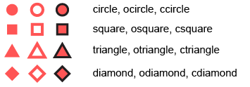
The non-primitive glyph types and their creator functions are:

| Type | R creator function |
| Text | l_glyph_add_text |
| Serialaxes | l_glyph_add_serialaxes |
| Pointranges | l_glyph_add_pointrange |
| Images | l_glyph_add_image |
| Polygon | l_glyph_add_polygon
|
When adding non-primitive glyphs to a display, the number of glyphs needs to
match the dimension n of the plot. In other words, a glyph needs to be
defined for each observations. See in the examples.
Currently loon does not support compound glyphs. However, it is possible to
cunstruct an arbitrary glyph using any system and save it as a png and then
re-import them as as image glyphs using l_glyph_add_image.
For more information run: l_help("learn_R_display_plot.html#glyphs")
Value
String with glyph id. Every set of non-primitive glyphs has an id (character).
See Also
l_glyph_add_text, l_make_glyphs
Other glyph functions:
l_glyph_add.default(),
l_glyph_add_image(),
l_glyph_add_pointrange(),
l_glyph_add_polygon(),
l_glyph_add_serialaxes(),
l_glyph_add_text(),
l_glyph_delete(),
l_glyph_getLabel(),
l_glyph_getType(),
l_glyph_ids(),
l_glyph_relabel(),
l_primitiveGlyphs()
Examples
if(interactive()){

# Simple Example with Text Glyphs
p <- with(olive, l_plot(stearic, eicosenoic, color=Region))
g <- l_glyph_add_text(p, text=olive$Area, label="Area")
p['glyph'] <- g

## Not run:
demo("l_glyphs", package="loon")

## End(Not run)

# create a plot that demonstrates the primitive glyphs and the text glyphs
p <- l_plot(x=1:15, y=rep(0,15), size=10, showLabels=FALSE)
text_glyph <- l_glyph_add_text(p, text=letters [1:15])
p['glyph'] <- c(
    'circle', 'ocircle', 'ccircle',
    'square', 'osquare' , 'csquare',
    'triangle', 'otriangle', 'ctriangle',
    'diamond', 'odiamond', 'cdiamond',
    rep(text_glyph, 3)
)
}
Default method for adding non-primitive glyphs
Description
Generic function to write new glyph types using loon's primitive glyphs
Usage
## Default S3 method:
l_glyph_add(widget, type, label = "", ...)
Arguments
widget |
widget path as a string or as an object handle |
type |
loon-native non-primitive glyph type, one of |
label |
label of a glyph (currently shown only in the glyph inspector) |
... |
state arguments |
See Also
Other glyph functions:
l_glyph_add(),
l_glyph_add_image(),
l_glyph_add_pointrange(),
l_glyph_add_polygon(),
l_glyph_add_serialaxes(),
l_glyph_add_text(),
l_glyph_delete(),
l_glyph_getLabel(),
l_glyph_getType(),
l_glyph_ids(),
l_glyph_relabel(),
l_primitiveGlyphs()
Add an image glyphs
Description
Image glyphs are useful to show pictures or other sophisticated compound glyphs. Note that images in the Tk canvas support transparancy.
Usage
l_glyph_add_image(widget, images, label = "", ...)
Arguments
widget |
widget path as a string or as an object handle |
images |
Tk image references, see the |
label |
label of a glyph (currently shown only in the glyph inspector) |
... |
state arguments |
Details
For more information run: l_help("learn_R_display_plot.html#images")
See Also
l_glyph_add, l_image_import_array,
l_image_import_files, l_make_glyphs
Other glyph functions:
l_glyph_add(),
l_glyph_add.default(),
l_glyph_add_pointrange(),
l_glyph_add_polygon(),
l_glyph_add_serialaxes(),
l_glyph_add_text(),
l_glyph_delete(),
l_glyph_getLabel(),
l_glyph_getType(),
l_glyph_ids(),
l_glyph_relabel(),
l_primitiveGlyphs()
Examples
if(interactive()){

p <- with(olive, l_plot(palmitic ~ stearic, color = Region))
img_paths <- list.files(file.path(find.package(package = 'loon'), "images"), full.names = TRUE)
imgs <- setNames(l_image_import_files(img_paths),
                 tools::file_path_sans_ext(basename(img_paths)))
i <- pmatch(gsub("^[[:alpha:]]+-","", olive$Area), names(imgs), duplicates.ok = TRUE)

g <- l_glyph_add_image(p, imgs[i], label="Flags")
p['glyph'] <- g
}
Add a Pointrange Glyph
Description
Pointrange glyphs show a filled circle at the x-y location and also a y-range.
Usage
l_glyph_add_pointrange(
  widget,
  ymin,
  ymax,
  linewidth = 1,
  showArea = TRUE,
  label = "",
  ...
)
Arguments
widget |
widget path as a string or as an object handle |
ymin |
vector with lower y-yalue of the point range. |
ymax |
vector with upper y-yalue of the point range. |
linewidth |
line with in pixel. |
showArea |
boolean, show a filled point or just the outline point |
label |
label of a glyph (currently shown only in the glyph inspector) |
... |
state arguments |
See Also
Other glyph functions:
l_glyph_add(),
l_glyph_add.default(),
l_glyph_add_image(),
l_glyph_add_polygon(),
l_glyph_add_serialaxes(),
l_glyph_add_text(),
l_glyph_delete(),
l_glyph_getLabel(),
l_glyph_getType(),
l_glyph_ids(),
l_glyph_relabel(),
l_primitiveGlyphs()
Examples
if(interactive()){

p <- l_plot(x = 1:3, color = c('red', 'blue', 'green'), showScales=TRUE)
g <- l_glyph_add_pointrange(p, ymin=(1:3)-(1:3)/5, ymax=(1:3)+(1:3)/5)
p['glyph'] <- g
}
Add a Polygon Glyph
Description
Add one polygon per scatterplot point.
Usage
l_glyph_add_polygon(
  widget,
  x,
  y,
  linewidth = 1,
  showArea = TRUE,
  label = "",
  ...
)
Arguments
widget |
widget path as a string or as an object handle |
x |
nested list of x-coordinates of polygons (relative to ), one list element for each scatterplot point. |
y |
nested list of y-coordinates of polygons, one list element for each scatterplot point. |
linewidth |
linewidth of outline. |
showArea |
boolean, show a filled polygon or just the outline |
label |
label of a glyph (currently shown only in the glyph inspector) |
... |
state arguments |
Details
A polygon can be a useful point glyph to visualize arbitrary shapes
such as airplanes, animals and shapes that are not available in the
primitive glyph types (e.g. cross). The l_glyphs demo has an example
of polygon glyphs which we reuse here.
See Also
Other glyph functions:
l_glyph_add(),
l_glyph_add.default(),
l_glyph_add_image(),
l_glyph_add_pointrange(),
l_glyph_add_serialaxes(),
l_glyph_add_text(),
l_glyph_delete(),
l_glyph_getLabel(),
l_glyph_getType(),
l_glyph_ids(),
l_glyph_relabel(),
l_primitiveGlyphs()
Examples
if(interactive()){

x_star <-
    c(-0.000864304235090734, 0.292999135695765, 0.949870354364736,
      0.474503025064823, 0.586862575626621, -0.000864304235090734,
      -0.586430423509075, -0.474070872947277, -0.949438202247191,
      -0.29256698357822)
y_star <-
    c(-1, -0.403630077787381, -0.308556611927398, 0.153846153846154,
      0.808556611927398, 0.499567847882455, 0.808556611927398,
      0.153846153846154, -0.308556611927398, -0.403630077787381)
x_cross <-
    c(-0.258931143762604, -0.258931143762604, -0.950374531835206,
      -0.950374531835206, -0.258931143762604, -0.258931143762604,
      0.259651397291847, 0.259651397291847, 0.948934024776722,
      0.948934024776722, 0.259651397291847, 0.259651397291847)
y_cross <-
    c(-0.950374531835206, -0.258931143762604, -0.258931143762604,
      0.259651397291847, 0.259651397291847, 0.948934024776722,
      0.948934024776722, 0.259651397291847, 0.259651397291847,
      -0.258931143762604, -0.258931143762604, -0.950374531835206)
x_hexagon <-
    c(0.773552290406223, 0, -0.773552290406223, -0.773552290406223,
      0, 0.773552290406223)
y_hexagon <-
    c(0.446917314894843, 0.894194756554307, 0.446917314894843,
      -0.447637568424085, -0.892754249495822, -0.447637568424085)

p <- l_plot(1:3, 1:3)

gl <- l_glyph_add_polygon(p, x = list(x_star, x_cross, x_hexagon),
                          y = list(y_star, y_cross, y_hexagon))

p['glyph'] <- gl

gl['showArea'] <- FALSE
}
Add a Serialaxes Glyph
Description
Serialaxes glyph show either a star glyph or a parallel coordinate glyph for each point.
Usage
l_glyph_add_serialaxes(
  widget,
  data,
  sequence,
  linewidth = 1,
  scaling = "variable",
  axesLayout = "radial",
  showAxes = FALSE,
  andrews = FALSE,
  axesColor = "gray70",
  showEnclosing = FALSE,
  bboxColor = "gray70",
  label = "",
  ...
)
Arguments
widget |
widget path as a string or as an object handle |
data |
a data frame with numerical data only |
sequence |
vector with variable names that defines the axes sequence |
linewidth |
linewidth of outline |
scaling |
one of 'variable', 'data', 'observation' or 'none' to specify how the data is scaled. See Details and Examples for more information. |
axesLayout |
either |
showAxes |
boolean to indicate whether axes should be shown or not |
andrews |
Andrew's curve (a 'Fourier' transformation) |
axesColor |
color of axes |
showEnclosing |
boolean, circle (axesLayout=radial) or sqaure (axesLayout=parallel) to show bounding box/circle of the glyph (or showing unit circle or rectangle with height 1 if scaling=none) |
bboxColor |
color of bounding box/circle |
label |
label of a glyph (currently shown only in the glyph inspector) |
... |
state arguments |
See Also
Other glyph functions:
l_glyph_add(),
l_glyph_add.default(),
l_glyph_add_image(),
l_glyph_add_pointrange(),
l_glyph_add_polygon(),
l_glyph_add_text(),
l_glyph_delete(),
l_glyph_getLabel(),
l_glyph_getType(),
l_glyph_ids(),
l_glyph_relabel(),
l_primitiveGlyphs()
Examples
if(interactive()){

p <- with(olive, l_plot(oleic, stearic, color=Area))
gs <- l_glyph_add_serialaxes(p, data=olive[,-c(1,2)], showArea=FALSE)
p['glyph'] <- gs
}
Add a Text Glyph
Description
Each text glyph can be a multiline string.
Usage
l_glyph_add_text(widget, text, label = "", ...)
Arguments
widget |
widget path as a string or as an object handle |
text |
the text strings for each observartion. If the object is a factor
then the labels get extracted with |
label |
label of a glyph (currently shown only in the glyph inspector) |
... |
state arguments |
See Also
Other glyph functions:
l_glyph_add(),
l_glyph_add.default(),
l_glyph_add_image(),
l_glyph_add_pointrange(),
l_glyph_add_polygon(),
l_glyph_add_serialaxes(),
l_glyph_delete(),
l_glyph_getLabel(),
l_glyph_getType(),
l_glyph_ids(),
l_glyph_relabel(),
l_primitiveGlyphs()
Examples
if(interactive()){

p <- l_plot(iris, color = iris$Species)
g <- l_glyph_add_text(p, iris$Species, "test_label")
p['glyph'] <- g
}
Delete a Glyph
Description
Delete a glyph from the plot.
Usage
l_glyph_delete(widget, id)
Arguments
widget |
widget path as a string or as an object handle |
id |
glyph id |
See Also
Other glyph functions:
l_glyph_add(),
l_glyph_add.default(),
l_glyph_add_image(),
l_glyph_add_pointrange(),
l_glyph_add_polygon(),
l_glyph_add_serialaxes(),
l_glyph_add_text(),
l_glyph_getLabel(),
l_glyph_getType(),
l_glyph_ids(),
l_glyph_relabel(),
l_primitiveGlyphs()
Get Glyph Label
Description
Returns the label of a glyph
Usage
l_glyph_getLabel(widget, id)
Arguments
widget |
widget path as a string or as an object handle |
id |
glyph id |
See Also
l_glyph_add, l_glyph_ids,
l_glyph_relabel
Other glyph functions:
l_glyph_add(),
l_glyph_add.default(),
l_glyph_add_image(),
l_glyph_add_pointrange(),
l_glyph_add_polygon(),
l_glyph_add_serialaxes(),
l_glyph_add_text(),
l_glyph_delete(),
l_glyph_getType(),
l_glyph_ids(),
l_glyph_relabel(),
l_primitiveGlyphs()
Get Glyph Type
Description
Query the type of a glyph
Usage
l_glyph_getType(widget, id)
Arguments
widget |
widget path as a string or as an object handle |
id |
glyph id |
See Also
Other glyph functions:
l_glyph_add(),
l_glyph_add.default(),
l_glyph_add_image(),
l_glyph_add_pointrange(),
l_glyph_add_polygon(),
l_glyph_add_serialaxes(),
l_glyph_add_text(),
l_glyph_delete(),
l_glyph_getLabel(),
l_glyph_ids(),
l_glyph_relabel(),
l_primitiveGlyphs()
List glyphs ids
Description
List all the non-primitive glyph ids attached to display.
Usage
l_glyph_ids(widget)
Arguments
widget |
widget path as a string or as an object handle |
See Also
Other glyph functions:
l_glyph_add(),
l_glyph_add.default(),
l_glyph_add_image(),
l_glyph_add_pointrange(),
l_glyph_add_polygon(),
l_glyph_add_serialaxes(),
l_glyph_add_text(),
l_glyph_delete(),
l_glyph_getLabel(),
l_glyph_getType(),
l_glyph_relabel(),
l_primitiveGlyphs()
Relabel Glyph
Description
Change the label of a glyph. Note that the label is only displayed in the glyph inspector.
Usage
l_glyph_relabel(widget, id, label)
Arguments
widget |
widget path as a string or as an object handle |
id |
glyph id |
label |
new label |
See Also
Other glyph functions:
l_glyph_add(),
l_glyph_add.default(),
l_glyph_add_image(),
l_glyph_add_pointrange(),
l_glyph_add_polygon(),
l_glyph_add_serialaxes(),
l_glyph_add_text(),
l_glyph_delete(),
l_glyph_getLabel(),
l_glyph_getType(),
l_glyph_ids(),
l_primitiveGlyphs()
Examples
if(interactive()){

p <- l_plot(iris, color = iris$Species)
g <- l_glyph_add_text(p, iris$Species, "test_label")
p['glyph'] <- g
l_glyph_relabel(p, g, "Species")
}
Create a Glyphs Inspector
Description
Inpectors provide graphical user interfaces to oversee and modify plot states
Usage
l_glyphs_inspector(parent = NULL, ...)
Arguments
parent |
parent widget path |
... |
state arguments |
Value
widget handle
See Also
Examples
if(interactive()){

i <- l_glyphs_inspector()
}
Create a Image Glyph Inspector
Description
Inpectors provide graphical user interfaces to oversee and modify plot states
Usage
l_glyphs_inspector_image(parent = NULL, ...)
Arguments
parent |
parent widget path |
... |
state arguments |
Value
widget handle
See Also
Examples
if(interactive()){

i <- l_glyphs_inspector_image()
}
Create a Pointrange Glyph Inspector
Description
Inpectors provide graphical user interfaces to oversee and modify plot states
Usage
l_glyphs_inspector_pointrange(parent = NULL, ...)
Arguments
parent |
parent widget path |
... |
state arguments |
Value
widget handle
See Also
Examples
if(interactive()){

i <- l_glyphs_inspector_pointrange()
}
Create a Serialaxes Glyph Inspector
Description
Inpectors provide graphical user interfaces to oversee and modify plot states
Usage
l_glyphs_inspector_serialaxes(parent = NULL, ...)
Arguments
parent |
parent widget path |
... |
state arguments |
Value
widget handle
See Also
Examples
if(interactive()){

i <- l_glyphs_inspector_serialaxes()
}
Create a Text Glyph Inspector
Description
Inpectors provide graphical user interfaces to oversee and modify plot states
Usage
l_glyphs_inspector_text(parent = NULL, ...)
Arguments
parent |
parent widget path |
... |
state arguments |
Value
widget handle
See Also
Examples
if(interactive()){

i <- l_glyphs_inspector_text()
}
Generic funtction to create an interactive graph display
Description
Interactive graphs in loon are currently most often used for navigation graphs.
Usage
l_graph(nodes, ...)

## S3 method for class 'graph'
l_graph(nodes, ...)

## S3 method for class 'loongraph'
l_graph(nodes, ...)

## Default S3 method:
l_graph(nodes = "", from = "", to = "", isDirected = FALSE, parent = NULL, ...)
Arguments
nodes |
object for method dispatch |
... |
arguments passed on to methods |
from |
vector with node names of the from-to pairs for edges |
to |
vector with node names of the from-to pairs for edges |
isDirected |
a boolean state to specify whether these edges have directions |
parent |
parent widget of graph display |
Details
For more information run: l_help("learn_R_display_graph.html#graph")
Value
graph handle
See Also
Other related graph objects, loongraph,
completegraph, linegraph,
complement, as.graph
Advanced usage l_navgraph,
l_ng_plots, l_ng_ranges
Examples
if(interactive()) {
 G <- completegraph(nodes=names(iris))
 LG <- linegraph(G, sep=":")
 g <- l_graph(LG)
}
Create a Graph Inspector
Description
Inpectors provide graphical user interfaces to oversee and modify plot states
Usage
l_graph_inspector(parent = NULL, ...)
Arguments
parent |
parent widget path |
... |
state arguments |
Value
widget handle
See Also
Examples
if(interactive()){

i <- l_graph_inspector()
}
Create a Graph Analysis Inspector
Description
Inpectors provide graphical user interfaces to oversee and modify plot states
Usage
l_graph_inspector_analysis(parent = NULL, ...)
Arguments
parent |
parent widget path |
... |
state arguments |
Value
widget handle
See Also
Examples
if(interactive()){

i <- l_graph_inspector_analysis()
}
Create a Graph Navigator Inspector
Description
Inpectors provide graphical user interfaces to oversee and modify plot states
Usage
l_graph_inspector_navigators(parent = NULL, ...)
Arguments
parent |
parent widget path |
... |
state arguments |
Value
widget handle
See Also
Examples
if(interactive()){

i <- l_graph_inspector_navigators()
}
Create a graphswitch widget
Description
The graphswitch provides a graphical user interface for changing the graph in a graph display interactively.
Usage
l_graphswitch(activewidget = "", parent = NULL, ...)
Arguments
activewidget |
widget handle of a graph display |
parent |
parent widget path |
... |
widget states |
Details
For more information run: l_help("learn_R_display_graph.html#graph-switch-widget")
See Also
l_graphswitch_add, l_graphswitch_ids,
l_graphswitch_delete, l_graphswitch_relabel,
l_graphswitch_getLabel, l_graphswitch_move,
l_graphswitch_reorder, l_graphswitch_set,
l_graphswitch_get
Add a graph to a graphswitch widget
Description
This is a generic function to add a graph to a graphswitch widget.
Usage
l_graphswitch_add(widget, graph, ...)
Arguments
widget |
widget path as a string or as an object handle |
graph |
a graph or a loongraph object |
... |
arguments passed on to method |
Details
For more information run: l_help("learn_R_display_graph.html#graph-switch-widget")
Value
id for graph in the graphswitch widget
See Also
Add a graph that is defined by node names and a from-to edges list
Description
This default method uses the loongraph display states as arguments to add a graph to the graphswitch widget.
Usage
## Default S3 method:
l_graphswitch_add(
  widget,
  graph,
  from,
  to,
  isDirected,
  label = "",
  index = "end",
  ...
)
Arguments
widget |
graphswitch widget handle (or widget path) |
graph |
a vector with the node names, i.e. this argument gets passed on
as the nodes argument to creat a |
from |
vector with node names of the from-to pairs for edges |
to |
vector with node names of the from-to pairs for edges |
isDirected |
boolean to indicate whether the from-to-list defines directed or undirected edges |
label |
string with label for graph |
index |
position of graph in the graph list |
... |
additional arguments are not used for this methiod |
Value
id for graph in the graphswitch widget
See Also
Add a graph to the graphswitch widget using a graph object
Description
Graph objects are defined in the graph R package.
Usage
## S3 method for class 'graph'
l_graphswitch_add(widget, graph, label = "", index = "end", ...)
Arguments
widget |
graphswitch widget handle (or widget path) |
graph |
a graph object created with the functions in the |
label |
string with label for graph |
index |
position of graph in the graph list |
... |
additional arguments are not used for this methiod |
Value
id for graph in the graphswitch widget
See Also
Add a graph to the graphswitch widget using a loongraph object
Description
Loongraphs can be created with the loongraph
function.
Usage
## S3 method for class 'loongraph'
l_graphswitch_add(widget, graph, label = "", index = "end", ...)
Arguments
widget |
graphswitch widget handle (or widget path) |
graph |
a loongraph object |
label |
string with label for graph |
index |
position of graph in the graph list |
... |
additional arguments are not used for this methiod |
Value
id for graph in the graphswitch widget
See Also
Delete a graph from the graphswitch widget
Description
Remove a a graph from the graphswitch widget
Usage
l_graphswitch_delete(widget, id)
Arguments
widget |
graphswitch widget handle (or widget path) |
id |
of the graph |
See Also
Return a Graph as a loongraph Object
Description
Graphs can be extracted from the graphswitch widget as loongraph objects.
Usage
l_graphswitch_get(widget, id)
Arguments
widget |
graphswitch widget handle (or widget path) |
id |
of the graph |
See Also
Query Label of a Graph in the Graphswitch Widget
Description
The graphs in the graphswitch widgets have labels. Use this function to query the label of a graph.
Usage
l_graphswitch_getLabel(widget, id)
Arguments
widget |
graphswitch widget handle (or widget path) |
id |
of the graph |
See Also
List the ids of the graphs in the graphswitch widget
Description
Every graph in the graphswitch widget has an id. This function returns these ids preserving the oder of how the graphs are listed in the graphswitch.
Usage
l_graphswitch_ids(widget)
Arguments
widget |
graphswitch widget handle (or widget path) |
Move a Graph in the Graph List
Description
Change the postion in of a graph in the graphswitch widget.
Usage
l_graphswitch_move(widget, id, index)
Arguments
widget |
graphswitch widget handle (or widget path) |
id |
of the graph |
index |
position of the graph as a positive integer, |
See Also
Relabel a Graph in the Graphswitch Widget
Description
The graphs in the graphswitch widgets have labels. Use this function the relabel a graph.
Usage
l_graphswitch_relabel(widget, id, label)
Arguments
widget |
graphswitch widget handle (or widget path) |
id |
of the graph |
label |
string with label of graph |
See Also
Reorder the Positions of the Graphs in the Graph List
Description
Define a new graph order in the graph list.
Usage
l_graphswitch_reorder(widget, ids)
Arguments
widget |
graphswitch widget handle (or widget path) |
ids |
vector with all graph ids from the graph widget. Use
|
See Also
Change the Graph shown in the Active Graph Widget
Description
The activewidget state holds the widget handle of a graph
display. This function replaces the graph in the activewidget with
one of the graphs in the graphswitch widget.
Usage
l_graphswitch_set(widget, id)
Arguments
widget |
graphswitch widget handle (or widget path) |
id |
of the graph |
See Also
Open a browser with loon's combined (TCL and R) documentation website
Description
l_help opens a browser with the relevant page on the
official combined loon documentation website at
https://great-northern-diver.github.io/loon/l_help/.
Usage
l_help(page = "index", ...)
Arguments
page |
relative path to a page, the .html part may be omitted |
... |
arguments forwarded to browseURL, e.g. to specify a browser |
See Also
help, l_web for R manual or
web R manual
Examples
## Not run:
l_help()
l_help("learn_R_intro")
l_help("learn_R_display_hist")
l_help("learn_R_bind")
# jump to a section
l_help("learn_R_bind.html#list-reorder-delete-bindings")

## End(Not run)
Convert color names to their 12 digit hexadecimal color representation
Description
Color names in loon will be mapped to colors according to the Tk color specifications and are normalized to a 12 digit hexadecimal color representation.
Usage
l_hexcolor(color)
Arguments
color |
a vector with color names |
Value
a character vector with the 12 digit hexadecimal color strings.
See Also
as_hex6color, hex12tohex6,
l_colorName
Examples
if(interactive()){

p <- l_plot(1:2)
p['color'] <- 'red'
p['color']

l_hexcolor('red')
}
Create an interactive histogram
Description
l_hist is a generic function for creating interactive histogram displays
that can be linked with loon's other displays.
Usage
l_hist(x, ...)

## Default S3 method:
l_hist(
  x,
  yshows = c("frequency", "density"),
  by = NULL,
  on,
  layout = c("grid", "wrap", "separate"),
  connectedScales = c("cross", "row", "column", "both", "x", "y", "none"),
  origin = NULL,
  binwidth = NULL,
  showStackedColors = TRUE,
  showBinHandle = FALSE,
  color = l_getOption("color"),
  active = TRUE,
  selected = FALSE,
  xlabel = NULL,
  showLabels = TRUE,
  showScales = FALSE,
  showGuides = TRUE,
  parent = NULL,
  ...
)

## S3 method for class 'factor'
l_hist(
  x,
  showFactors = length(unique(x)) < 25L,
  factorLabelAngle,
  factorLabelSize = 12,
  factorLabelColor = l_getOption("foreground"),
  factorLabelY = 0,
  ...
)

## S3 method for class 'character'
l_hist(
  x,
  showFactors = length(unique(x)) < 25L,
  factorLabelAngle,
  factorLabelSize = 12,
  factorLabelColor = l_getOption("foreground"),
  factorLabelY = 0,
  ...
)

## S3 method for class 'data.frame'
l_hist(x, ...)

## S3 method for class 'matrix'
l_hist(x, ...)

## S3 method for class 'list'
l_hist(x, ...)

## S3 method for class 'table'
l_hist(x, ...)

## S3 method for class 'array'
l_hist(x, ...)
Arguments
x |
vector with numerical data to perform the binning on x, |
... |
named arguments to modify the histogram plot states or layouts, see details. |
yshows |
one of "frequency" (default) or "density" |
by |
loon plot can be separated by some variables into multiple panels.
This argument can take a |
on |
if the |
layout |
layout facets as |
connectedScales |
Determines how the scales of the facets are to be connected depending
on which
|
origin |
numeric scalar to define the binning origin |
binwidth |
a numeric scalar to specify the binwidth
If NULL |
showStackedColors |
if TRUE (default) then bars will be coloured according to colours of the points; if FALSE, then the bars will be a uniform colour except for highlighted points. |
showBinHandle |
If |
color |
colour fills of bins; colours are repeated
until matching the number x.
Default is found using |
active |
a logical determining whether points appear or not
(default is |
selected |
a logical determining whether points appear selected at first
(default is |
xlabel |
label to be used on the horizontal axis. If NULL, an attempt at a meaningful label
inferred from |
showLabels |
logical to determine whether axes label (and title) should be presented. |
showScales |
logical to determine whether numerical scales should be presented on both axes. |
showGuides |
logical to determine whether to present background guidelines to help determine locations. |
parent |
a valid Tk parent widget path. When the parent widget is
specified (i.e. not |
showFactors |
whether to show the factor labels (unique strings in |
factorLabelAngle |
is the angle of rotation (in degrees) for the factor labels. If not specified, an angle of 0 is chosen if there are fewer than 10 labels; labels are rotated 90 degrees if there are 10 or more. This can also be a numeric vector of length equal to the number of factor labels. |
factorLabelSize |
is the font size for the factor labels (default 12). |
factorLabelColor |
is the colour to be used for the factor labels.
(default is |
factorLabelY |
either a single number, or a numeric vector of length equal to the number of factor labels, determining the y coordinate(s) for the factor labels. |
Details
For more information run: l_help("learn_R_display_hist")
-
Note that when changing the
yshowsstate from'frequency'to'density'you might have to usel_scaleto_worldto show the complete histogram in the plotting region. -
Some arguments to modify layouts can be passed through, e.g. "separate", "byrow", etc. Check
l_facetto see how these arguments work.
Value
if the argument by is not set, a loon widget will be returned;
else an l_facet object (a list) will be returned and each element is
a loon widget displaying a subset of interest.
See Also
Turn interactive loon plot static loonGrob, grid.loon, plot.loon.
Other loon interactive states:
l_info_states(),
l_plot(),
l_serialaxes(),
l_state_names(),
names.loon()
Examples
if(interactive()){

h <- l_hist(iris$Sepal.Length)

names(h)
h["xlabel"] <- "Sepal length"
h["showOutlines"] <- FALSE

h["yshows"]
h["yshows"] <- "density"
l_scaleto_plot(h)

h["showStackedColors"] <- TRUE
h['color'] <- iris$Species
h["showStackedColors"] <- FALSE
h["showOutlines"] <- TRUE
h["showGuides"] <- FALSE

# link another plot with the previous plot
h['linkingGroup'] <- "iris_data"
h2 <- with(iris, l_hist(Petal.Width,
                        linkingGroup="iris_data",
                        showStackedColors = TRUE))


# Get an R (grid) graphics plot of the current loon plot
plot(h)
# or with more control about grid parameters
grid.loon(h)
# or to save the grid data structure (grob) for later use
hg <- loonGrob(h)

}
Create a Histogram Inspector
Description
Inpectors provide graphical user interfaces to oversee and modify plot states
Usage
l_hist_inspector(parent = NULL, ...)
Arguments
parent |
parent widget path |
... |
state arguments |
Value
widget handle
See Also
Examples
if(interactive()){

i <- l_hist_inspector()
}
Create a Histogram Analysis Inspector
Description
Inpectors provide graphical user interfaces to oversee and modify plot states
Usage
l_hist_inspector_analysis(parent = NULL, ...)
Arguments
parent |
parent widget path |
... |
state arguments |
Value
widget handle
See Also
Examples
if(interactive()){

i <- l_hist_inspector_analysis()
}
Import Greyscale Images as Tcl images from an Array
Description
Import image grayscale data (0-255) with each image saved as a row or column of an array.
Usage
l_image_import_array(
  array,
  width,
  height,
  img_in_row = TRUE,
  invert = FALSE,
  rotate = 0
)
Arguments
array |
of 0-255 grayscale value data. |
width |
of images in pixels. |
height |
of images in pixels. |
img_in_row |
logical, TRUE if every row of the array represents an image |
invert |
logical, for 'invert=FALSE' 0=withe, for 'invert=TRUE' 0=black |
rotate |
the image: one of 0, 90, 180, or 270 degrees. |
Details
Images in tcl are managed by the tcl interpreter and made accessible to the user via a handle, i.e. a function name of the form image1, image2, etc.
For more information run: l_help("learn_R_display_plot.html#images")
Value
vector of image object names
Examples
## Not run:
# see
demo("l_ng_images_frey_LLE")

## End(Not run)
Import Image Files as Tk Image Objects
Description
Note that the supported image file formats depend on whether the
Img Tk extension is installed.
Usage
l_image_import_files(paths)
Arguments
paths |
vector with paths to image files that are supported |
Details
For more information run: l_help("learn_R_display_plot.html#load-images")
Value
vector of image object names
See Also
l_image_import_array, l_imageviewer
Display Tcl Images in a Simple Image Viewer
Description
Loon provides a simple image viewer to browse through the specified tcl image objects.
The simple GUI supports either the use of the mouse or left and right arrow keys to switch the images to the previous or next image in the specified image vector.
The images are resized to fill the viewer window.
Usage
l_imageviewer(tclimages)
Arguments
tclimages |
Vector of tcl image object names. |
Value
the tclimages vector is returned
Examples
if(interactive()){


img2 <- tkimage.create('photo', width=200, height=150)
tcl(img2, 'put', 'yellow', '-to', 0, 0, 199, 149)
tcl(img2, 'put', 'green', '-to', 40, 20, 130, 40)
img3 <- tkimage.create('photo', width=500, height=100)
tcl(img3, 'put', 'orange', '-to', 0, 0, 499, 99)
tcl(img3, 'put', 'green', '-to', 40, 80, 350, 95)

l_imageviewer(c(tclvalue(img2), tclvalue(img3)))

}
Retrieve Information about the States of a Loon Widget
Description
Loon's built-in object documentation. Can be used with every loon object that has plot states including plots, layers, navigators, contexts. This is a generic function.
Usage
l_info_states(target, states = "all")
Arguments
target |
either an object of class loon or a vector that specifies the
widget, layer, glyph, navigator or context completely. The widget is
specified by the widget path name (e.g. |
states |
vector with names of states. |
Value
a named nested list with one element per state. The list elements are
also named lists with type, dimension, defaultvalue,
and description elements containing the respective information.
See Also
Other loon interactive states:
l_hist(),
l_plot(),
l_serialaxes(),
l_state_names(),
names.loon()
Examples
if(interactive()){

p <- l_plot(iris, linkingGroup="iris")
i <- l_info_states(p)
names(p)
names(i)
i$selectBy

l <- l_layer_rectangle(p, x=range(iris[,1]), y=range(iris[,2]), color="")
l_info_states(l)


h <- l_hist(iris$Sepal.Length, linkingGroup="iris")
l_info_states(h)

}
Check if a widget path is a valid loon widget
Description
This function can be useful to check whether a loon widget is has been closed by the user.
Usage
l_isLoonWidget(widget)
Arguments
widget |
widget path as a string or as an object handle |
Value
boolean, TRUE if the argument is a valid loon widget path, FALSE otherwise
Loon layers
Description
Loon supports layering of visuals and groups of visuals. The
l_layer function is a generic method.
Usage
l_layer(widget, x, ...)
Arguments
widget |
widget path as a string or as an object handle |
x |
for |
... |
additional arguments, often state definition for the basic layering function |
Details
loon's displays that use the main graphics model (i.e. histogram, scatterplot and graph displays) support layering of visual information. The following table lists the layer types and functions for layering on a display.
| Type | Description | Creator Function |
| group | a group can be a parent of other layers |
l_layer_group |
| polygon | one polygon |
l_layer_polygon |
| text | one text string |
l_layer_text |
| line | one line (i.e. connected line segments) | l_layer_line |
| rectangle | one rectangle | l_layer_rectangle |
| oval | one oval |
l_layer_oval |
| points | n points (filled) circle |
l_layer_points |
| texts | n text strings |
l_layer_text |
| polygons | n polygons |
l_layer_polygons |
| rectangles | n rectangles |
l_layer_rectangles |
| lines | n sets of connected line segments | l_layer_lines |
| smooth | fitted smooth line | l_layer_smooth |
| rasterImage | one raster image | l_layer_rasterImage |
| heatImage | one heat image | l_layer_heatImage |
| contourLines | contour lines | l_layer_contourLines |
Every layer within a display has a unique id. The visuals of the data in a
display present the default layer of that display and has the layer id
'model'. For example, the 'model' layer of a scatterplot
display visualizes the scatterplot glyphs. Functions useful to query layers
are
| Function | Description |
l_layer_ids | List layer ids |
l_layer_getType | Get layer type |
Layers are arranged in a tree structure with the tree root having the layer
id 'root'. The rendering order of the layers is according to a
depth-first traversal of the layer tree. This tree also maintains a label
and a visibility flag for each layer. The layer tree, layer ids, layer
labels and the visibility of each layer are visualized in the layers
inspector. If a layer is set to be invisible then it is not rendered on the
display. If a group layer is set to be invisible then all its children are
not rendered; however, the visibility flag of the children layers remain
unchanged. Relevant functions are:
| Function | Description |
l_layer_getParent | Get parent layer id of a layer |
l_layer_getChildren | Get children of a group layer |
l_layer_index | Get the order index of a layer among its siblings |
l_layer_printTree | Print out the layer tree |
l_layer_move | Move a layer |
l_layer_lower | Switch the layer place with its sibling to the right |
l_layer_raise | Switch the layer place with its sibling to the left |
l_layer_demote | Moves the layer up to be a left sibling of its parent |
l_layer_promote | Moves the layer to be a child of its right group layer sibling |
l_layer_hide | Set the
layers visibility flag to FALSE |
l_layer_show |
Set the layers visibility flag to TRUE |
l_layer_isVisible | Return visibility flag of layer |
l_layer_layerVisibility | Returns logical value for whether layer is actually seen |
l_layer_groupVisibility
| Returns all, part or none for expressing which
part of the layers children are visible. |
l_layer_delete
| Delete a layer. If the layer is a group move all its children layers to the layers parent. |
l_layer_expunge | Delete layer and all its children layer. |
l_layer_getLabel | Get layer label. |
l_layer_relabel | Change layer label. |
l_layer_bbox | Get the bounding box of a layer. |
All layers have states that can be queried and modified using the same
functions as the ones used for displays (i.e. l_cget,
l_configure, `[` and `[<-`). The
last group of layer types in the above table have n-dimensional states,
where the actual value of n can be different for every layer in a display.
The difference between the model layer and the other layers is that the model layer has a selected state, responds to selection gestures and supports linking.
For more information run: l_help("learn_R_layer")
Value
layer object handle, layer id
See Also
l_info_states, l_scaleto_layer, l_scaleto_world;
some l_layer S3 methods:
l_layer.density, l_layer.map,
l_layer.SpatialPolygonsDataFrame, l_layer.SpatialPolygons,
l_layer.Polygons, l_layer.Polygon, l_layer.SpatialLinesDataFrame,
l_layer.SpatialLines, l_layer.Lines, l_layer.Line,
l_layer.SpatialPointsDataFrame, l_layer.SpatialPoints
Examples
if(interactive()){

# l_layer is a generic method
newFoo <- function(x, y, ...) {
  r <- list(x=x, y=y, ...)
  class(r) <- 'foo'
  return(r)
}

l_layer.foo <- function(widget, x) {
    x$widget <- widget
    id <- do.call('l_layer_polygon', x)
    return(id)
}

p <- l_plot()

obj <- newFoo(x=c(1:6,6:2), y=c(3,1,0,0,1,3,3,5,6,6,5), color='yellow')

id <- l_layer(p, obj)

l_scaleto_world(p)
}
Layer line in Line object
Description
Methods to plot map data defined in the sp
package
Usage
## S3 method for class 'Line'
l_layer(widget, x, ...)
Arguments
widget |
widget widget path as a string or as an object handle |
x |
an object defined in the |
... |
arguments forwarded to the relative |
Details
Note that currently loon does neither support holes and ring directions.
Value
layer id
References
Applied Spatial Data Analysis with R by Bivand, Roger S. and Pebesma, Edzer and Gomez-Rubio and Virgilio
See Also
Examples
if (interactive()) {

if (requireNamespace("rworldmap", quietly = TRUE)) {
    world <- rworldmap::getMap(resolution = "coarse")
    p <- l_plot()
    lmap <- l_layer(p, world, asSingleLayer=TRUE)
    l_scaleto_world(p)
    attr(lmap,'hole')
    attr(lmap,'NAME')
}
}
Layer lines in Lines object
Description
Methods to plot map data defined in the sp
package
Usage
## S3 method for class 'Lines'
l_layer(widget, x, asSingleLayer = TRUE, ...)
Arguments
widget |
widget widget path as a string or as an object handle |
x |
an object defined in the |
asSingleLayer |
If |
... |
arguments forwarded to the relative |
Details
Note that currently loon does neither support holes and ring directions.
Value
layer id
References
Applied Spatial Data Analysis with R by Bivand, Roger S. and Pebesma, Edzer and Gomez-Rubio and Virgilio
See Also
Examples
if (interactive()) {

if (requireNamespace("rworldmap", quietly = TRUE)) {
    world <- rworldmap::getMap(resolution = "coarse")
    p <- l_plot()
    lmap <- l_layer(p, world, asSingleLayer=TRUE)
    l_scaleto_world(p)
    attr(lmap,'hole')
    attr(lmap,'NAME')
}
}
Layer polygon in Polygon object
Description
Methods to plot map data defined in the sp
package
Usage
## S3 method for class 'Polygon'
l_layer(widget, x, ...)
Arguments
widget |
widget widget path as a string or as an object handle |
x |
an object defined in the |
... |
arguments forwarded to the relative |
Details
Note that currently loon does neither support holes and ring directions.
Value
layer id
References
Applied Spatial Data Analysis with R by Bivand, Roger S. and Pebesma, Edzer and Gomez-Rubio and Virgilio
See Also
Examples
if (interactive()) {

if (requireNamespace("rworldmap", quietly = TRUE)) {
    world <- rworldmap::getMap(resolution = "coarse")
    p <- l_plot()
    lmap <- l_layer(p, world, asSingleLayer=TRUE)
    l_scaleto_world(p)
    attr(lmap,'hole')
    attr(lmap,'NAME')
}
}
Layer polygons in Polygons object
Description
Methods to plot map data defined in the sp
package
Usage
## S3 method for class 'Polygons'
l_layer(widget, x, asSingleLayer = TRUE, ...)
Arguments
widget |
widget widget path as a string or as an object handle |
x |
an object defined in the |
asSingleLayer |
If |
... |
arguments forwarded to the relative |
Details
Note that currently loon does neither support holes and ring directions.
Value
layer id
References
Applied Spatial Data Analysis with R by Bivand, Roger S. and Pebesma, Edzer and Gomez-Rubio and Virgilio
See Also
Examples
if (interactive()) {

if (requireNamespace("rworldmap", quietly = TRUE)) {
    world <- rworldmap::getMap(resolution = "coarse")
    p <- l_plot()
    lmap <- l_layer(p, world, asSingleLayer=TRUE)
    l_scaleto_world(p)
    attr(lmap,'hole')
    attr(lmap,'NAME')
}
}
Layer lines in SpatialLines object
Description
Methods to plot map data defined in the sp
package
Usage
## S3 method for class 'SpatialLines'
l_layer(widget, x, asSingleLayer = TRUE, ...)
Arguments
widget |
widget widget path as a string or as an object handle |
x |
an object defined in the |
asSingleLayer |
If |
... |
arguments forwarded to the relative |
Details
Note that currently loon does neither support holes and ring directions.
Value
layer id
References
Applied Spatial Data Analysis with R by Bivand, Roger S. and Pebesma, Edzer and Gomez-Rubio and Virgilio
See Also
Examples
if (interactive()) {

if (requireNamespace("rworldmap", quietly = TRUE)) {
    world <- rworldmap::getMap(resolution = "coarse")
    p <- l_plot()
    lmap <- l_layer(p, world, asSingleLayer=TRUE)
    l_scaleto_world(p)
    attr(lmap,'hole')
    attr(lmap,'NAME')
}
}
Layer lines in SpatialLinesDataFrame object
Description
Methods to plot map data defined in the sp
package
Usage
## S3 method for class 'SpatialLinesDataFrame'
l_layer(widget, x, asSingleLayer = TRUE, ...)
Arguments
widget |
widget widget path as a string or as an object handle |
x |
an object defined in the |
asSingleLayer |
If |
... |
arguments forwarded to the relative |
Details
Note that currently loon does neither support holes and ring directions.
Value
layer id
References
Applied Spatial Data Analysis with R by Bivand, Roger S. and Pebesma, Edzer and Gomez-Rubio and Virgilio
See Also
Examples
if (interactive()) {

if (requireNamespace("rworldmap", quietly = TRUE)) {
    world <- rworldmap::getMap(resolution = "coarse")
    p <- l_plot()
    lmap <- l_layer(p, world, asSingleLayer=TRUE)
    l_scaleto_world(p)
    attr(lmap,'hole')
    attr(lmap,'NAME')
}
}
Layer points in SpatialPoints object
Description
Methods to plot map data defined in the sp
package
Usage
## S3 method for class 'SpatialPoints'
l_layer(widget, x, asMainLayer = FALSE, ...)
Arguments
widget |
widget widget path as a string or as an object handle |
x |
an object defined in the |
asMainLayer |
if |
... |
arguments forwarded to the relative |
Details
Note that currently loon does neither support holes and ring directions.
Value
layer id
References
Applied Spatial Data Analysis with R by Bivand, Roger S. and Pebesma, Edzer and Gomez-Rubio and Virgilio
See Also
Examples
if (interactive()) {

if (requireNamespace("rworldmap", quietly = TRUE)) {
    world <- rworldmap::getMap(resolution = "coarse")
    p <- l_plot()
    lmap <- l_layer(p, world, asSingleLayer=TRUE)
    l_scaleto_world(p)
    attr(lmap,'hole')
    attr(lmap,'NAME')
}
}
Layer points in SpatialPointsDataFrame object
Description
Methods to plot map data defined in the sp
package
Usage
## S3 method for class 'SpatialPointsDataFrame'
l_layer(widget, x, asMainLayer = FALSE, ...)
Arguments
widget |
widget widget path as a string or as an object handle |
x |
an object defined in the |
asMainLayer |
if |
... |
arguments forwarded to the relative |
Details
Note that currently loon does neither support holes and ring directions.
Value
layer id
References
Applied Spatial Data Analysis with R by Bivand, Roger S. and Pebesma, Edzer and Gomez-Rubio and Virgilio
See Also
Examples
if (interactive()) {

if (requireNamespace("rworldmap", quietly = TRUE)) {
    world <- rworldmap::getMap(resolution = "coarse")
    p <- l_plot()
    lmap <- l_layer(p, world, asSingleLayer=TRUE)
    l_scaleto_world(p)
    attr(lmap,'hole')
    attr(lmap,'NAME')
}
}
Layer polygons in SpatialPolygons object
Description
Methods to plot map data defined in the sp
package
Usage
## S3 method for class 'SpatialPolygons'
l_layer(widget, x, asSingleLayer = TRUE, ...)
Arguments
widget |
widget widget path as a string or as an object handle |
x |
an object defined in the |
asSingleLayer |
If |
... |
arguments forwarded to the relative |
Details
Note that currently loon does neither support holes and ring directions.
Value
layer id
References
Applied Spatial Data Analysis with R by Bivand, Roger S. and Pebesma, Edzer and Gomez-Rubio and Virgilio
See Also
Examples
if (interactive()) {

if (requireNamespace("rworldmap", quietly = TRUE)) {
    world <- rworldmap::getMap(resolution = "coarse")
    p <- l_plot()
    lmap <- l_layer(p, world, asSingleLayer=TRUE)
    l_scaleto_world(p)
    attr(lmap,'hole')
    attr(lmap,'NAME')
}
}
Layer polygons in SpatialPolygonDataFrame
Description
Methods to plot map data defined in the sp
package
Usage
## S3 method for class 'SpatialPolygonsDataFrame'
l_layer(widget, x, asSingleLayer = TRUE, ...)
Arguments
widget |
widget widget path as a string or as an object handle |
x |
an object defined in the |
asSingleLayer |
If |
... |
arguments forwarded to the relative |
Details
Note that currently loon does neither support holes and ring directions.
Value
layer id
References
Applied Spatial Data Analysis with R by Bivand, Roger S. and Pebesma, Edzer and Gomez-Rubio and Virgilio
See Also
Examples
if (interactive()) {

if (requireNamespace("rworldmap", quietly = TRUE)) {
    world <- rworldmap::getMap(resolution = "coarse")
    p <- l_plot()
    lmap <- l_layer(p, world, asSingleLayer=TRUE)
    l_scaleto_world(p)
    attr(lmap,'hole')
    attr(lmap,'NAME')
}
}
Layer Method for Kernel Density Estimation
Description
Layer a line that represents a kernel density estimate.
Usage
## S3 method for class 'density'
l_layer(widget, x, ...)
Arguments
widget |
widget path as a string or as an object handle |
x |
object from |
... |
additional arguments, often state definition for the basic layering function |
Value
layer object handle, layer id
See Also
Examples
if(interactive()){
  d <- density(faithful$eruptions, bw = "sj")
  h <- l_hist(x = faithful$eruptions, yshows="density")
  l <- l_layer.density(h, d, color="steelblue", linewidth=3)
  # or l <- l_layer(h, d, color="steelblue", linewidth=3)
}
Add a Map of class map as Drawings to Loon plot
Description
The maps library provides some map data in polygon which can be added as drawings (currently with polygons) to Loon plots. This function adds map objects with class map from the maps library as background drawings.
Usage
## S3 method for class 'map'
l_layer(
  widget,
  x,
  color = "",
  linecolor = "black",
  linewidth = 1,
  label,
  parent = "root",
  index = 0,
  asSingleLayer = TRUE,
  ...
)
Arguments
widget |
widget path as a string or as an object handle |
x |
a map object of class |
color |
fill color, if empty string |
linecolor |
outline color |
linewidth |
linewidth of outline |
label |
label used in the layers inspector |
parent |
a valid Tk parent widget path. When the parent widget is
specified (i.e. not |
index |
position among its siblings. valid values are 0, 1, 2, ..., 'end' |
asSingleLayer |
if |
... |
additional arguments are not used for this methiod |
Value
If asSingleLayer=TRUE then returns layer id of polygons layer,
otherwise group layer that contains polygon children layers.
Examples
if(interactive()){

if (requireNamespace("maps", quietly = TRUE)) {
  canada <- maps::map("world",  "Canada",
                      fill=TRUE, plot=FALSE)
  p <- l_plot()
  l_map <- l_layer(p, canada,
                   asSingleLayer=TRUE, color = "cornsilk")
  l_map['color'] <- ifelse(grepl("lake", canada$names, TRUE),
                           "lightblue", "cornsilk")
  l_scaleto_layer(p, l_map)
  l_map['active'] <- FALSE
  l_map['active'] <- TRUE
  l_map['tag']
}

}
Get the bounding box of a layer.
Description
The bounding box of a layer returns the coordinates of the smallest rectangle that encloses all the elements of the layer.
Usage
l_layer_bbox(widget, layer = "root")
Arguments
widget |
widget path or layer object of class |
layer |
layer id. If the widget argument is of class |
Value
Numeric vector of length 4 with (xmin, ymin, xmax, ymax) of the bounding box
Examples
if(interactive()){

p <- with(iris, l_plot(Sepal.Length ~ Sepal.Width, color=Species))
l_layer_bbox(p, layer='model')

l <- l_layer_rectangle(p, x=0:1, y=30:31)
l_layer_bbox(p, l)

l_layer_bbox(p, 'root')

}
Layer Contour Lines
Description
This function is a wrapper around
contourLines that adds the countourlines to a loon
plot which is based on the cartesian coordinate system.
Usage
l_layer_contourLines(
  widget,
  x = seq(0, 1, length.out = nrow(z)),
  y = seq(0, 1, length.out = ncol(z)),
  z,
  nlevels = 10,
  levels = pretty(range(z, na.rm = TRUE), nlevels),
  asSingleLayer = TRUE,
  parent = "root",
  index = "end",
  ...
)
Arguments
widget |
widget path as a string or as an object handle |
x, y |
As described in |
z |
As described in |
nlevels |
As described in |
levels |
As described in |
asSingleLayer |
if |
parent |
a valid Tk parent widget path. When the parent widget is
specified (i.e. not |
index |
position among its siblings. valid values are 0, 1, 2, ..., 'end' |
... |
arguments forwarded to |
Details
For more information run: l_help("learn_R_layer.html#countourlines-heatimage-rasterimage")
Value
layer id of group or lines layer
Examples
if(interactive()){

p <- l_plot()
x <- 10*1:nrow(volcano)
y <- 10*1:ncol(volcano)
lcl <- l_layer_contourLines(p, x, y, volcano)
l_scaleto_world(p)

if (requireNamespace("MASS", quietly = TRUE)) {

  p1 <- with(iris, l_plot(Sepal.Length~Sepal.Width, color=Species))
  lcl <- with(iris, l_layer_contourLines(p1, MASS::kde2d(Sepal.Width,Sepal.Length)))

  p2 <- with(iris, l_plot(Sepal.Length~Sepal.Width, color=Species))
  layers <- sapply(split(cbind(iris, color=p2['color']), iris$Species), function(dat) {
       kest <- with(dat, MASS::kde2d(Sepal.Width,Sepal.Length))
       l_layer_contourLines(p2, kest, color=as.character(dat$color[1]), linewidth=2,
            label=paste0(as.character(dat$Species[1]), " contours"))
  })
}

}
Delete a layer
Description
All but the 'model' and the 'root' layer can be
dynamically deleted. If a group layer gets deleted with
l_layer_delete then all its children layers get moved into their
grandparent group layer.
Usage
l_layer_delete(widget, layer)
Arguments
widget |
widget path or layer object of class |
layer |
layer id. If the widget argument is of class |
Value
0 if success otherwise the function throws an error
See Also
Examples
if(interactive()){

p <- l_plot()
l1 <- l_layer_rectangle(p, x = 0:1, y = 0:1, color='red')
l_layer_delete(l1)

l2 <- l_layer_rectangle(p, x = 0:1, y = 0:1, color='yellow')
l_layer_delete(p,l2)

}
Moves the layer to be a child of its right group layer sibling
Description
Moves the layer up the layer tree (away from the root layer) if there is a sibling group layer to the right of the layer.
Usage
l_layer_demote(widget, layer)
Arguments
widget |
widget path or layer object of class |
layer |
layer id. If the widget argument is of class |
Value
0 if success otherwise the function throws an error
Examples
if(interactive()){

p <- l_plot()

g1 <- l_layer_group(p)
g2 <- l_layer_group(p, parent=g1)
l1 <- l_layer_oval(p, x=0:1, y=0:1)

l_layer_printTree(p)
l_layer_demote(p, l1)
l_layer_printTree(p)
l_layer_demote(p, l1)
l_layer_printTree(p)

}
Delete a layer and all its descendants
Description
Delete a group layer and all it's descendants. Note that the
'model' layer cannot be deleted.
Usage
l_layer_expunge(widget, layer)
Arguments
widget |
widget path or layer object of class |
layer |
layer id. If the widget argument is of class |
Value
0 if success otherwise the function throws an error
See Also
Examples
if(interactive()){

p <- l_plot()
g <- l_layer_group(p)
l1 <- l_layer_rectangle(p, x=0:1, y=0:1, parent=g, color="", linecolor="orange", linewidth=2)
l2 <- l_layer_line(p, x=c(0,.5,1), y=c(0,1,0), parent=g, color="blue")

l_layer_expunge(p, g)

# or l_layer_expunge(g)

}
Get children of a group layer
Description
Returns the ids of a group layer's children.
Usage
l_layer_getChildren(widget, layer = "root")
Arguments
widget |
widget path or layer object of class |
layer |
layer id. If the widget argument is of class |
Value
Character vector with ids of the childrens. To create layer handles
(i.e. objects of class 'l_layer') use the
l_create_handle function.
See Also
Examples
if(interactive()){

p <- l_plot()

g <- l_layer_group(p)
l1 <- l_layer_rectangle(p, x=0:1, y=0:1, parent=g)
l2 <- l_layer_oval(p, x=0:1, y=0:1, color='thistle', parent=g)

l_layer_getChildren(p, g)

}
Get layer label.
Description
Layer labels are useful to identify layer in the layer inspector. The layer label can be initially set at layer creation with the label argument.
Usage
l_layer_getLabel(widget, layer)
Arguments
widget |
widget path or layer object of class |
layer |
layer id. If the widget argument is of class |
Details
Note that the layer label is not a state of the layer itself, instead is information that is part of the layer collection (i.e. its parent widget).
Value
Named vector of length 1 with layer label as value and layer id as name.
See Also
Examples
if(interactive()){

p <- l_plot()
l1 <- l_layer_rectangle(p, x=0:1, y=0:1, label="a rectangle")
l_layer_getLabel(p, 'model')
l_layer_getLabel(p, l1)

}
Get parent layer id of a layer
Description
The toplevel parent is the 'root' layer.
Usage
l_layer_getParent(widget, layer)
Arguments
widget |
widget path or layer object of class |
layer |
layer id. If the widget argument is of class |
See Also
Examples
if(interactive()){

p <- with(iris, l_plot(Sepal.Length ~ Sepal.Width, color=Species))

l_layer_getParent(p, 'model')

}
Get layer type
Description
To see the manual page of l_layer for all the
primitive layer types.
Usage
l_layer_getType(widget, layer)
Arguments
widget |
widget path or layer object of class |
layer |
layer id. If the widget argument is of class |
Details
For more information run: l_help("learn_R_layer")
Value
One of: 'group', 'polygon', 'text',
'line', 'rectangle', 'oval', 'points',
'texts', 'polygons', 'rectangles', 'lines' and
'scatterplot', 'histogram', 'serialaxes' and
'graph'.
See Also
Examples
if(interactive()){

p <- l_plot()
l <- l_layer_rectangle(p, x=0:1, y=0:1)
l_layer_getType(p, l)
l_layer_getType(p, 'model')

}
layer a group node
Description
Loon's displays that are based on Cartesian coordinates (i.e. scatterplot, histogram and graph display) allow for layering visual information including polygons, text and rectangles.
A group layer can contain other layers. If the group layer is invisible, then so are all its children.
Usage
l_layer_group(widget, label = "group", parent = "root", index = 0)
Arguments
widget |
widget path name as a string |
label |
label used in the layers inspector |
parent |
group layer |
index |
of the newly added layer in its parent group |
Details
For more information run: l_help("learn_R_layer")
Value
layer object handle, layer id
See Also
Examples
if (interactive()){
p <- l_plot(x=c(1,10,1.5,7,4.3,9,5,2,8),
             y=c(1,10,7,3,4,3.3,8,3,4),
             title="Demo Layers")

id.g <- l_layer_group(p, "A Layer Group")
id.pts <- l_layer_points(p, x=c(3,6), y=c(4,7), color="red", parent=id.g)
l_scaleto_layer(p, id.pts)
l_configure(id.pts, x=c(-5,5,12), y=c(-2,-5,18), color="lightgray")

}
Queries visibility status of decendants
Description
Query whether all, part or none of the group layers descendants are visible.
Usage
l_layer_groupVisibility(widget, layer)
Arguments
widget |
widget path or layer object of class |
layer |
layer id. If the widget argument is of class |
Details
Visibile layers are rendered, invisible ones are not. If any
ancestor of a layer is set to be invisible then the layer is not rendered
either. The layer visibility flag can be checked with
l_layer_isVisible and the actual visibility (i.e. are all the
ancesters visibile too) can be checked with
l_layer_layerVisibility.
Note that layer visibility is not a state of the layer itself, instead is information that is part of the layer collection (i.e. its parent widget).
Value
'all', 'part' or 'none' depending on the
visibility status of the descendants.
See Also
l_layer, l_layer_show,
l_layer_hide, l_layer_isVisible,
l_layer_layerVisibility
Examples
if(interactive()){

p <- l_plot()

g <- l_layer_group(p)
l1 <- l_layer_rectangle(p, x=0:1, y=0:1, parent=g)
l2 <- l_layer_oval(p, x=0:1, y=0:1, parent=g)

l_layer_groupVisibility(p, g)
l_layer_hide(p, l2)
l_layer_groupVisibility(p, g)
l_layer_hide(p, l1)
l_layer_groupVisibility(p, g)
l_layer_hide(p, g)
l_layer_groupVisibility(p, g)

}
Display a Heat Image
Description
This function is very similar to the
image function. It works with every loon plot which
is based on the cartesian coordinate system.
Usage
l_layer_heatImage(
  widget,
  x = seq(0, 1, length.out = nrow(z)),
  y = seq(0, 1, length.out = ncol(z)),
  z,
  zlim = range(z[is.finite(z)]),
  xlim = range(x),
  ylim = range(y),
  col = grDevices::heat.colors(12),
  breaks,
  oldstyle = FALSE,
  useRaster,
  index = "end",
  parent = "root",
  ...
)
Arguments
widget |
widget path as a string or as an object handle |
x |
locations of grid lines at which the values in z are measured. These must be finite, non-missing and in (strictly) ascending order. By default, equally spaced values from 0 to 1 are used. If x is a list, its components x$x and x$y are used for x and y, respectively. If the list has component z this is used for z. |
y |
see description for the |
z |
a numeric or logical matrix containing the values to be plotted
( |
zlim |
the minimum and maximum |
xlim |
range for the plotted x values, defaulting to the range of x |
ylim |
range for the plotted y values, defaulting to the range of y |
col |
a list of colors such as that generated by
|
breaks |
a set of finite numeric breakpoints for the colours: must have one more breakpoint than colour and be in increasing order. Unsorted vectors will be sorted, with a warning. |
oldstyle |
logical. If true the midpoints of the colour intervals
are equally spaced, and |
useRaster |
logical; if |
index |
position among its siblings. valid values are 0, 1, 2, ..., 'end' |
parent |
a valid Tk parent widget path. When the parent widget is
specified (i.e. not |
... |
argumnets forwarded to |
Details
For more information run: l_help("learn_R_layer.html#countourlines-heatimage-rasterimage")
Value
layer id of group or rectangles layer
Examples
if(interactive()){

if (requireNamespace("MASS", quietly = TRUE)) {
  kest <- with(iris, MASS::kde2d(Sepal.Width,Sepal.Length))
  image(kest)
  contour(kest, add=TRUE)

  p <- l_plot()
  lcl <- l_layer_contourLines(p, kest, label='contour lines')
  limg <- l_layer_heatImage(p, kest, label='heatmap')
  l_scaleto_world(p)
}

# from examples(image)
x <- y <- seq(-4*pi, 4*pi, len = 27)
r <- sqrt(outer(x^2, y^2, "+"))
p1 <- l_plot()
l_layer_heatImage(p1, z = z <- cos(r^2)*exp(-r/6), col  = gray((0:32)/32))
l_scaleto_world(p1)

image(z = z <- cos(r^2)*exp(-r/6), col  = gray((0:32)/32))

}
Hide a Layer
Description
A hidden layer is not rendered. If a group layer is set to be hidden then all its descendants are not rendered either.
Usage
l_layer_hide(widget, layer)
Arguments
widget |
widget path or layer object of class |
layer |
layer id. If the widget argument is of class |
Details
Visibile layers are rendered, invisible ones are not. If any
ancestor of a layer is set to be invisible then the layer is not rendered
either. The layer visibility flag can be checked with
l_layer_isVisible and the actual visibility (i.e. are all the
ancesters visibile too) can be checked with
l_layer_layerVisibility.
Note that layer visibility is not a state of the layer itself, instead is information that is part of the layer collection (i.e. its parent widget).
Value
0 if success otherwise the function throws an error
See Also
l_layer, l_layer_show,
l_layer_isVisible, l_layer_layerVisibility,
l_layer_groupVisibility
Examples
if(interactive()){

p <- l_plot()

l <- l_layer_rectangle(p, x=0:1, y=0:1, color="steelblue")
l_layer_hide(p, l)

}
List ids of layers in Plot
Description
Every layer within a display has a unique id. This function returns a list of all the layer ids for a widget.
Usage
l_layer_ids(widget)
Arguments
widget |
widget path as a string or as an object handle |
Details
For more information run: l_help("learn_R_layer.html#add-move-delete-layers")
Value
vector with layer ids in rendering order. To create a layer handle
object use l_create_handle.
See Also
Examples
if (interactive()){
set.seed(500)
x <- rnorm(30)
y <- 4 + 3*x + rnorm(30)
fit <- lm(y~x)
xseq <- seq(min(x)-1, max(x)+1, length.out = 50)
fit_line <- predict(fit, data.frame(x=range(xseq)))
ci <- predict(fit, data.frame(x=xseq),
              interval="confidence", level=0.95)
pi <- predict(fit, data.frame(x=xseq),
              interval="prediction", level=0.95)


p <- l_plot(y~x, color='black', showScales=TRUE, showGuides=TRUE)
gLayer <- l_layer_group(
    p, label="simple linear regression",
    parent="root", index="end"
)
fitLayer <- l_layer_line(
    p, x=range(xseq), y=fit_line, color="#04327F",
    linewidth=4, label="fit", parent=gLayer
)
ciLayer <- l_layer_polygon(
    p,
    x = c(xseq, rev(xseq)),
    y = c(ci[,'lwr'], rev(ci[,'upr'])),
    color = "#96BDFF", linecolor="",
    label = "95 % confidence interval",
    parent = gLayer, index='end'
)
piLayer <- l_layer_polygon(
    p,
    x = c(xseq, rev(xseq)),
    y = c(pi[,'lwr'], rev(pi[,'upr'])),
    color = "#E2EDFF", linecolor="",
    label = "95 % prediction interval",
    parent = gLayer, index='end'
)

l_info_states(piLayer)

}
Get the order index of a layer among its siblings
Description
The index determines the rendering order of the children layers of a parent. The layer with index=0 is rendered first.
Usage
l_layer_index(widget, layer)
Arguments
widget |
widget path or layer object of class |
layer |
layer id. If the widget argument is of class |
Details
Note that the index for layers is 0 based.
Value
numeric value
See Also
Return visibility flag of layer
Description
Hidden or invisible layers are not rendered. This function queries whether a layer is visible/rendered or not.
Usage
l_layer_isVisible(widget, layer)
Arguments
widget |
widget path or layer object of class |
layer |
layer id. If the widget argument is of class |
Details
Visibile layers are rendered, invisible ones are not. If any
ancestor of a layer is set to be invisible then the layer is not rendered
either. The layer visibility flag can be checked with
l_layer_isVisible and the actual visibility (i.e. are all the
ancesters visibile too) can be checked with
l_layer_layerVisibility.
Note that layer visibility is not a state of the layer itself, instead is information that is part of the layer collection (i.e. its parent widget).
Value
TRUE or FALSE depending whether the layer is visible or
not.
See Also
l_layer, l_layer_show,
l_layer_hide, l_layer_layerVisibility,
l_layer_groupVisibility
Examples
if(interactive()){

p <- l_plot()
l <- l_layer_rectangle(p, x=0:1, y=0:1)
l_layer_isVisible(p, l)
l_layer_hide(p, l)
l_layer_isVisible(p, l)

}
Returns logical value for whether layer is actually seen
Description
Although the visibility flag for a layer might be set to
TRUE it won't be rendered as on of its ancestor group layer is set
to be invisible. The l_layer_visibility returns TRUE if the
layer and all its ancestor layers have their visibility flag set to true
and the layer is actually rendered.
Usage
l_layer_layerVisibility(widget, layer)
Arguments
widget |
widget path or layer object of class |
layer |
layer id. If the widget argument is of class |
Details
Visibile layers are rendered, invisible ones are not. If any
ancestor of a layer is set to be invisible then the layer is not rendered
either. The layer visibility flag can be checked with
l_layer_isVisible and the actual visibility (i.e. are all the
ancesters visibile too) can be checked with
l_layer_layerVisibility.
Note that layer visibility is not a state of the layer itself, instead is information that is part of the layer collection (i.e. its parent widget).
Value
TRUE if the layer and all its ancestor layers have their
visibility flag set to true and the layer is actually rendered, otherwise
FALSE.
See Also
l_layer, l_layer_show,
l_layer_hide, l_layer_isVisible,
l_layer_groupVisibility
Layer a line
Description
Loon's displays that are based on Cartesian coordinates (i.e. scatterplot, histogram and graph display) allow for layering visual information including polygons, text and rectangles.
Usage
l_layer_line(
  widget,
  x,
  y = NULL,
  color = "black",
  linewidth = 1,
  dash = "",
  label = "line",
  parent = "root",
  index = 0,
  ...
)
Arguments
widget |
widget path name as a string |
x |
the coordinates of line. Alternatively, a single plotting structure,
function or any R object with a plot method can be provided as x and
y are passed on to |
y |
the y coordinates of the line, optional if x is an appropriate structure. |
color |
color of line |
linewidth |
linewidth of outline |
dash |
dash pattern of line, see https://www.tcl-lang.org/man/tcl8.6/TkCmd/canvas.htm#M26 |
label |
label used in the layers inspector |
parent |
group layer |
index |
of the newly added layer in its parent group |
... |
additional state initialization arguments, see
|
Details
For more information run: l_help("learn_R_layer")
Value
layer object handle, layer id
See Also
Examples
if(interactive()){

p <- l_plot()
l <- l_layer_line(p, x=c(1,2,3,4), y=c(1,3,2,4), color='red', linewidth=2)
l_scaleto_world(p)

# object
p <- l_plot()
l <- l_layer_line(p, x=nhtemp)
l_scaleto_layer(l)

}
Layer lines
Description
Loon's displays that are based on Cartesian coordinates (i.e. scatterplot, histogram and graph display) allow for layering visual information including polygons, text and rectangles.
Usage
l_layer_lines(
  widget,
  x,
  y,
  color = "black",
  linewidth = 1,
  label = "lines",
  parent = "root",
  index = 0,
  group = NULL,
  active = TRUE,
  ...
)
Arguments
widget |
widget path name as a string |
x |
list with vectors with x coordinates |
y |
list with vectors with y coordinates |
color |
color of lines |
linewidth |
vector with line widths |
label |
label used in the layers inspector |
parent |
group layer |
index |
of the newly added layer in its parent group |
group |
separate x vector or y vector into a list by group. |
active |
a logical determining whether objects appear or not
(default is |
... |
additional state initialization arguments, see
|
Details
For more information run: l_help("learn_R_layer")
Value
layer object handle, layer id
See Also
Examples
if(interactive()){

s <- Filter(function(df)nrow(df) > 1, split(UsAndThem, UsAndThem$Country))
sUaT <- Map(function(country){country[order(country$Year),]} , s)
xcoords <- Map(function(x)x$Year, sUaT)
ycoords <- Map(function(x)x$LifeExpectancy, sUaT)
region <- sapply(sUaT, function(x)as.character(x$Geographic.Region[1]))

p <- l_plot(showItemLabels=TRUE)
l <- l_layer_lines(p, xcoords, ycoords, itemLabel=names(sUaT), color=region)
l_scaleto_layer(l)

# Set groups
p <- l_plot(showItemLabels=TRUE)
l <- l_layer_lines(p,
                   x = c((0:4)/10, rep(.5, 5), (10:6)/10, rep(.5, 5)),
                   y = c(rep(.5, 5), (10:6/10), rep(.5, 5), (0:4)/10),
                   group = rep(1:5, 4),
                   linewidth = 4,
                   col = l_getColorList()[1:5])
l_scaleto_layer(l)

}
Switch the layer place with its sibling to the right
Description
Change the layers position within its parent layer group by
increasing the index of the layer by one if possible. This means
that the raised layer will be rendered before (or on below) of its sibling
layer to the right.
Usage
l_layer_lower(widget, layer)
Arguments
widget |
widget path or layer object of class |
layer |
layer id. If the widget argument is of class |
Value
0 if success otherwise the function throws an error
See Also
l_layer, l_layer_raise, l_layer_move
Examples
if(interactive()){

p <- l_plot()

l1 <- l_layer_rectangle(p, x=0:1, y=0:1)
l2 <- l_layer_oval(p, x=0:1, y=0:1, color='thistle')

l_aspect(p) <- 1

l_layer_lower(p, l2)

}
Move a layer
Description
The postition of a layer in the layer tree determines the
rendering order. That is, the non-group layers are rendered in order of a
Depth-first traversal of the layer tree. The toplevel group layer is called
'root'.
Usage
l_layer_move(widget, layer, parent, index = "0")
Arguments
widget |
widget path or layer object of class |
layer |
layer id. If the widget argument is of class |
parent |
if parent layer is not specified it is set to the current parent layer of the layer |
index |
position among its siblings. valid values are 0, 1, 2, ..., 'end' |
Value
0 if success otherwise the function throws an error
See Also
l_layer, l_layer_printTree,
l_layer_index
Examples
if(interactive()){

p <- l_plot()

l <- l_layer_rectangle(p, x=0:1, y=0:1, color="steelblue")
g <- l_layer_group(p)
l_layer_printTree(p)

l_layer_move(l, parent=g)
l_layer_printTree(p)

l_layer_move(p, 'model', parent=g)
l_layer_printTree(p)

}
Layer a oval
Description
Loon's displays that are based on Cartesian coordinates (i.e. scatterplot, histogram and graph display) allow for layering visual information including polygons, text and rectangles.
Usage
l_layer_oval(
  widget,
  x,
  y,
  color = "gray80",
  linecolor = "black",
  linewidth = 1,
  label = "oval",
  parent = "root",
  index = 0,
  ...
)
Arguments
widget |
widget path name as a string |
x |
x coordinates |
y |
y coordinates |
color |
fill color, if empty string |
linecolor |
outline color |
linewidth |
linewidth of outline |
label |
label used in the layers inspector |
parent |
group layer |
index |
of the newly added layer in its parent group |
... |
additional state initialization arguments, see
|
Details
For more information run: l_help("learn_R_layer")
Value
layer object handle, layer id
See Also
Examples
if(interactive()){

p <- l_plot()
l <- l_layer_oval(p, c(1,5), c(2,12), color='steelblue')
l_configure(p, panX=0, panY=0, deltaX=20, deltaY=20)

}
Layer points
Description
Loon's displays that are based on Cartesian coordinates (i.e. scatterplot, histogram and graph display) allow for layering visual information including polygons, text and rectangles.
Scatter points layer
Usage
l_layer_points(
  widget,
  x,
  y = NULL,
  color = "gray60",
  size = 6,
  label = "points",
  parent = "root",
  index = 0,
  active = TRUE,
  ...
)
Arguments
widget |
widget path name as a string |
x |
the coordinates of line. Alternatively, a single plotting structure,
function or any R object with a plot method can be provided as x and
y are passed on to |
y |
the y coordinates of the line, optional if x is an appropriate structure. |
color |
color of points |
size |
size point, as for scatterplot model layer |
label |
label used in the layers inspector |
parent |
group layer |
index |
of the newly added layer in its parent group |
active |
a logical determining whether objects appear or not
(default is |
... |
additional state initialization arguments, see
|
Details
For more information run: l_help("learn_R_layer")
Value
layer object handle, layer id
See Also
Layer a polygon
Description
Loon's displays that are based on Cartesian coordinates (i.e. scatterplot, histogram and graph display) allow for layering visual information including polygons, text and rectangles.
Usage
l_layer_polygon(
  widget,
  x,
  y,
  color = "gray80",
  linecolor = "black",
  linewidth = 1,
  label = "polygon",
  parent = "root",
  index = 0,
  ...
)
Arguments
widget |
widget path name as a string |
x |
x coordinates |
y |
y coordinates |
color |
fill color, if empty string |
linecolor |
outline color |
linewidth |
linewidth of outline |
label |
label used in the layers inspector |
parent |
group layer |
index |
of the newly added layer in its parent group |
... |
additional state initialization arguments, see
|
Details
For more information run: l_help("learn_R_layer")
Value
layer object handle, layer id
See Also
Examples
if (interactive()){
set.seed(500)
x <- rnorm(30)
y <- 4 + 3*x + rnorm(30)
fit <- lm(y~x)
xseq <- seq(min(x)-1, max(x)+1, length.out = 50)
fit_line <- predict(fit, data.frame(x=range(xseq)))
ci <- predict(fit, data.frame(x=xseq),
              interval="confidence", level=0.95)
pi <- predict(fit, data.frame(x=xseq),
              interval="prediction", level=0.95)


p <- l_plot(y~x, color='black', showScales=TRUE, showGuides=TRUE)
gLayer <- l_layer_group(
    p, label="simple linear regression",
    parent="root", index="end"
)
fitLayer <- l_layer_line(
    p, x=range(xseq), y=fit_line, color="#04327F",
    linewidth=4, label="fit", parent=gLayer
)
ciLayer <- l_layer_polygon(
    p,
    x = c(xseq, rev(xseq)),
    y = c(ci[,'lwr'], rev(ci[,'upr'])),
    color = "#96BDFF", linecolor="",
    label = "95 % confidence interval",
    parent = gLayer, index='end'
)
piLayer <- l_layer_polygon(
    p,
    x = c(xseq, rev(xseq)),
    y = c(pi[,'lwr'], rev(pi[,'upr'])),
    color = "#E2EDFF", linecolor="",
    label = "95 % prediction interval",
    parent = gLayer, index='end'
)

l_info_states(piLayer)

}
Layer polygons
Description
Loon's displays that are based on Cartesian coordinates (i.e. scatterplot, histogram and graph display) allow for layering visual information including polygons, text and rectangles.
Usage
l_layer_polygons(
  widget,
  x,
  y,
  color = "gray80",
  linecolor = "black",
  linewidth = 1,
  label = "polygons",
  parent = "root",
  index = 0,
  group = NULL,
  active = TRUE,
  ...
)
Arguments
widget |
widget path name as a string |
x |
list with vectors with x coordinates |
y |
list with vectors with y coordinates |
color |
vector with fill colors, if empty string |
linecolor |
vector with outline colors |
linewidth |
vector with line widths |
label |
label used in the layers inspector |
parent |
group layer |
index |
of the newly added layer in its parent group |
group |
separate x vector or y vector into a list by group. |
active |
a logical determining whether objects appear or not
(default is |
... |
additional state initialization arguments, see
|
Details
For more information run: l_help("learn_R_layer")
Value
layer object handle, layer id
See Also
Examples
if(interactive()){

p <- l_plot()

l <- l_layer_polygons(
     p,
     x = list(c(1,2,1.5), c(3,4,6,5,2), c(1,3,5,3)),
     y = list(c(1,1,2), c(1,1.5,1,4,2), c(3,5,6,4)),
     color = c('red', 'green', 'blue'),
     linecolor = ""
)
l_scaleto_world(p)

l_info_states(l, "color")


# Set groups
p <- l_plot()
l_layer_polygons(p,
                 x = c(1, 2, 1.5, 3, 4, 6, 5, 2, 1, 3, 5, 3),
                 y = c(1, 1, 2, 1, 1.5, 1, 4, 2, 3, 5, 6, 4),
                 group = c(rep(1,3), rep(2,5), rep(3, 4)))
l_scaleto_world(p)

}
Print the layer tree
Description
Prints the layer tree (i.e. the layer ids) to the prompt. Group
layers are prefixed with a '+'. The 'root' layer is not
listed.
Usage
l_layer_printTree(widget)
Arguments
widget |
widget path as a string or as an object handle |
Value
empty string
See Also
l_layer, l_layer_getChildren, l_layer_getParent
Examples
if(interactive()){

p <- l_plot()
l_layer_rectangle(p, x=0:1, y=0:1)
g <- l_layer_group(p)
l_layer_oval(p, x=0:1, y=0:1, parent=g)
l_layer_line(p, x=0:1, y=0:1, parent=g)
l_layer_printTree(p)

}
Moves the layer up to be a left sibling of its parent
Description
Moves the layer down the layer tree (towards the root layer) if the parent layer is not the root layer.
Usage
l_layer_promote(widget, layer)
Arguments
widget |
widget path or layer object of class |
layer |
layer id. If the widget argument is of class |
Value
0 if success otherwise the function throws an error
Examples
if(interactive()){

p <- l_plot()

g1 <- l_layer_group(p)
g2 <- l_layer_group(p, parent=g1)
l1 <- l_layer_oval(p, x=0:1, y=0:1, parent=g2)

l_layer_printTree(p)
l_layer_promote(p, l1)
l_layer_printTree(p)
l_layer_promote(p, l1)
l_layer_printTree(p)

}
Switch the layer place with its sibling to the left
Description
Change the layers position within its parent layer group by
decreasing the index of the layer by one if possible. This means
that the raised layer will be rendered after (or on top) of its sibling
layer to the left.
Usage
l_layer_raise(widget, layer)
Arguments
widget |
widget path or layer object of class |
layer |
layer id. If the widget argument is of class |
Value
0 if success otherwise the function throws an error
See Also
l_layer, l_layer_lower, l_layer_move
Examples
if(interactive()){

p <- l_plot()

l1 <- l_layer_rectangle(p, x=0:1, y=0:1)
l2 <- l_layer_oval(p, x=0:1, y=0:1, color='thistle')

l_aspect(p) <- 1

l_layer_raise(p, l1)

}
Layer a Raster Image
Description
This function is very similar to the
rasterImage function. It works with every loon plot
which is based on the cartesian coordinate system.
Usage
l_layer_rasterImage(
  widget,
  image,
  xleft,
  ybottom,
  xright,
  ytop,
  angle = 0,
  interpolate = FALSE,
  parent = "root",
  index = "end",
  ...
)
Arguments
widget |
widget path as a string or as an object handle |
image |
a |
xleft |
a vector (or scalar) of left x positions. |
ybottom |
a vector (or scalar) of bottom y positions. |
xright |
a vector (or scalar) of right x positions. |
ytop |
a vector (or scalar) of top y positions. |
angle |
angle of rotation (in degrees, anti-clockwise from positive x-axis, about the bottom-left corner). |
interpolate |
a logical vector (or scalar) indicating whether to apply linear interpolation to the image when drawing. |
parent |
a valid Tk parent widget path. When the parent widget is
specified (i.e. not |
index |
position among its siblings. valid values are 0, 1, 2, ..., 'end' |
... |
argumnets forwarded to |
Details
For more information run: l_help("learn_R_layer.html#countourlines-heatimage-rasterimage")
Value
layer id of group or rectangles layer
Examples
if(interactive()){

plot(1,1, xlim = c(0,1), ylim=c(0,1))
mat <- matrix(c(0,0,0,0, 1,1), ncol=2)
rasterImage(mat, 0,0,1,1, interpolate = FALSE)

p <- l_plot()
l_layer_rasterImage(p, mat, 0,0,1,1)
l_scaleto_world(p)

image <- as.raster(matrix(0:1, ncol = 5, nrow = 3))
p <- l_plot(showScales=TRUE, background="thistle", useLoonInspector=FALSE)
l_layer_rasterImage(p, image, 100, 300, 150, 350, interpolate = FALSE)
l_layer_rasterImage(p, image, 100, 400, 150, 450)
l_layer_rasterImage(p, image, 200, 300, 200 + 10, 300 + 10,
   interpolate = FALSE)
l_scaleto_world(p)

# from examples(rasterImage)

# set up the plot region:
op <- par(bg = "thistle")
plot(c(100, 250), c(300, 450), type = "n", xlab = "", ylab = "")
rasterImage(image, 100, 300, 150, 350, interpolate = FALSE)
rasterImage(image, 100, 400, 150, 450)
rasterImage(image, 200, 300, 200 + 10, 300 + 10,
           interpolate = FALSE)

}
Layer a rectangle
Description
Loon's displays that are based on Cartesian coordinates (i.e. scatterplot, histogram and graph display) allow for layering visual information including polygons, text and rectangles.
Usage
l_layer_rectangle(
  widget,
  x,
  y,
  color = "gray80",
  linecolor = "black",
  linewidth = 1,
  label = "rectangle",
  parent = "root",
  index = 0,
  ...
)
Arguments
widget |
widget path name as a string |
x |
x coordinates |
y |
y coordinates |
color |
fill color, if empty string |
linecolor |
outline color |
linewidth |
linewidth of outline |
label |
label used in the layers inspector |
parent |
group layer |
index |
of the newly added layer in its parent group |
... |
additional state initialization arguments, see
|
Details
For more information run: l_help("learn_R_layer")
Value
layer object handle, layer id
See Also
Examples
if(interactive()){

p <- l_plot()
l <- l_layer_rectangle(p, x=c(2,3), y=c(1,10), color='steelblue')
l_scaleto_layer(l)

}
Layer rectangles
Description
Loon's displays that are based on Cartesian coordinates (i.e. scatterplot, histogram and graph display) allow for layering visual information including polygons, text and rectangles.
Usage
l_layer_rectangles(
  widget,
  x,
  y,
  color = "gray80",
  linecolor = "black",
  linewidth = 1,
  label = "rectangles",
  parent = "root",
  index = 0,
  group = NULL,
  active = TRUE,
  ...
)
Arguments
widget |
widget path name as a string |
x |
list with vectors with x coordinates |
y |
list with vectors with y coordinates |
color |
vector with fill colors, if empty string |
linecolor |
vector with outline colors |
linewidth |
vector with line widths |
label |
label used in the layers inspector |
parent |
group layer |
index |
of the newly added layer in its parent group |
group |
separate x vector or y vector into a list by group. |
active |
a logical determining whether objects appear or not
(default is |
... |
additional state initialization arguments, see
|
Details
For more information run: l_help("learn_R_layer")
Value
layer object handle, layer id
See Also
Examples
if(interactive()){

p <- l_plot()

l <- l_layer_rectangles(
     p,
     x = list(c(0,1), c(1,2), c(2,3), c(5,6)),
     y = list(c(0,1), c(1,2), c(0,1), c(3,4)),
     color = c('red', 'blue', 'green', 'orange'),
     linecolor = "black"
)
l_scaleto_world(p)

l_info_states(l)

# Set groups
pp <- l_plot(x = c(0,1,1,2,2,3,5,6),
             y = c(0,1,1,2,0,1,3,4))
# x and y are inherited from pp
ll <- l_layer_rectangles(
     pp,
     group = rep(1:4, each = 2),
     color = c('red', 'blue', 'green', 'orange'),
     linecolor = "black"
)
l_scaleto_world(pp)

}
Change layer label
Description
Layer labels are useful to identify layer in the layer inspector. The layer label can be initially set at layer creation with the label argument.
Usage
l_layer_relabel(widget, layer, label)
Arguments
widget |
widget path or layer object of class |
layer |
layer id. If the widget argument is of class |
label |
new label of layer |
Details
Note that the layer label is not a state of the layer itself, instead is information that is part of the layer collection (i.e. its parent widget).
Value
0 if success otherwise the function throws an error
See Also
Examples
if(interactive()){

p <- l_plot()

l <- l_layer_rectangle(p, x=0:1, y=0:1, label="A rectangle")
l_layer_getLabel(p, l)

l_layer_relabel(p, l, label="A relabelled rectangle")
l_layer_getLabel(p, l)

}
Show or unhide a Layer
Description
Hidden or invisible layers are not rendered. This function unhides invisible layer so that they are rendered again.
Usage
l_layer_show(widget, layer)
Arguments
widget |
widget path or layer object of class |
layer |
layer id. If the widget argument is of class |
Details
Visibile layers are rendered, invisible ones are not. If any
ancestor of a layer is set to be invisible then the layer is not rendered
either. The layer visibility flag can be checked with
l_layer_isVisible and the actual visibility (i.e. are all the
ancesters visibile too) can be checked with
l_layer_layerVisibility.
Note that layer visibility is not a state of the layer itself, instead is information that is part of the layer collection (i.e. its parent widget).
Value
0 if success otherwise the function throws an error
See Also
l_layer, l_layer_hide,
l_layer_isVisible, l_layer_layerVisibility,
l_layer_groupVisibility
Examples
if(interactive()){

p <- l_plot()

l <- l_layer_rectangle(p, x=0:1, y=0:1, color="steelblue")
l_layer_hide(p, l)

l_layer_show(p, l)

}
Layer a smooth line for loon
Description
Display a smooth line layer
Usage
l_layer_smooth(
  widget,
  x = NULL,
  y = NULL,
  method = "loess",
  group = "",
  formula = y ~ x,
  interval = c("none", "confidence", "prediction"),
  n = 80,
  span = 0.75,
  level = 0.95,
  methodArgs = list(),
  linecolor = "steelblue",
  linewidth = 2,
  linedash = "",
  confidenceIntervalArgs = list(linecolor = "gray80", linewidth = 4, linedash = ""),
  predictionIntervalArgs = list(linecolor = "gray50", linewidth = 3, linedash = 1),
  label = "smooth",
  parent = "root",
  index = 0,
  ...
)
Arguments
widget |
widget path name as a string |
x |
The |
y |
The |
method |
Smoothing method (function) to use, accepts either a character vector, e.g. "lm", "glm", "loess" or a function, e.g. MASS::rlm or mgcv::gam, stats::lm, or stats::loess. |
group |
Data can be grouped by n dimensional aesthetics attributes, e.g. "color", "size". In addition, any length n vector or data.frame is accommodated. |
formula |
Formula to use in smoothing function, eg. y ~ x, y ~ poly(x, 2), y ~ log(x) |
interval |
type of interval, could be "none", "confidence" or "prediction" (not for |
n |
Number of points at which to evaluate smoother. |
span |
Controls the amount of smoothing for the default |
level |
Level of confidence interval to use (0.95 by default). |
methodArgs |
List of additional arguments passed on to the modelling function defined by method. |
linecolor |
fitted line color. |
linewidth |
fitted line width |
linedash |
fitted line dash |
confidenceIntervalArgs |
the line color, width and dash for confidence interval |
predictionIntervalArgs |
the line color, width and dash for prediction interval |
label |
label used in the layers inspector |
parent |
group layer |
index |
index of the newly added layer in its parent group |
... |
additional state initialization arguments, see |
Examples
if(interactive()) {
# loess fit
p <- l_plot(iris, color = iris$Species)
l1 <- l_layer_smooth(p, interval = "confidence")
l_layer_hide(l1)

# the fits are grouped by points color
l2 <- l_layer_smooth(p, group = "color",
                     method = "lm")

# so far, all intervals are hidden
ls <- l_layer_getChildren(l2)
intervals <- l_layer_getChildren(l_create_handle(c(p,ls[3])))
ci <- l_create_handle(c(p,intervals[3]))
l_layer_show(ci)
# show prediction interval
pi <- l_create_handle(c(p,intervals[2]))
l_layer_show(pi)
# hide all
l_layer_hide(l2)

# Draw a fitted line based on a new data set
shortSepalLength <- (iris$Sepal.Length < 5)
l3 <- l_layer_smooth(p,
                     x = iris$Sepal.Length[shortSepalLength],
                     y = iris$Sepal.Width[shortSepalLength],
                     method = "lm",
                     linecolor = "firebrick",
                     interval = "prediction")
l_layer_hide(l3)

if(require(mgcv)) {
  # a full tensor product smooth
  ## linecolor is the same with the points color
  l4 <- l_layer_smooth(p,
                       method = "gam",
                       formula = y~te(x))
  l_layer_hide(l4)
}

# facets
fp <- l_facet(p, by = iris$Species, inheritLayers = FALSE)
l5 <- l_layer_smooth(fp, method = "lm")

# generalized linear model
if(require("loon.data")) {
  data("SAheart")
  # logit regression
  chd <- as.numeric(SAheart$chd) - 1
  age <- SAheart$age
  p1 <- l_plot(age, chd,
               title = "logit regression")
  gl1 <- l_layer_smooth(p1,
                        method = "glm",
                        methodArgs = list(family = binomial()),
                        interval = "conf")

  # log linear regression
  counts <- c(18,17,15,20,10,20,25,13,12)
  age <- c(40,35,53,46,20,33,48,25,23)
  p2 <- l_plot(age, counts,
               title = "log-linear regression")
  gl2 <- l_layer_smooth(p2,
                        method = "glm",
                        methodArgs = list(family = poisson()),
                        interval = "conf")
}
}
Layer a text
Description
Loon's displays that are based on Cartesian coordinates (i.e. scatterplot, histogram and graph display) allow for layering visual information including polygons, text and rectangles.
layer a single character string
Usage
l_layer_text(
  widget,
  x,
  y,
  text,
  color = "gray60",
  size = 6,
  angle = 0,
  label = "text",
  parent = "root",
  index = 0,
  ...
)
Arguments
widget |
widget path name as a string |
x |
coordinate |
y |
coordinate |
text |
character string |
color |
color of text |
size |
size of the font |
angle |
rotation of text |
label |
label used in the layers inspector |
parent |
group layer |
index |
of the newly added layer in its parent group |
... |
additional state initialization arguments, see
|
Details
As a side effect of Tcl's text-based design, it is best to
use l_layer_text if one would like to layer a single character
string (and not l_layer_texts with n=1).
For more information run: l_help("learn_R_layer")
Value
layer object handle, layer id
See Also
Examples
if(interactive()){

p <- l_plot()
l <- l_layer_text(p, 0, 0, "Hello World")

}
Layer texts
Description
Loon's displays that are based on Cartesian coordinates (i.e. scatterplot, histogram and graph display) allow for layering visual information including polygons, text and rectangles.
Layer a vector of character strings.
Usage
l_layer_texts(
  widget,
  x,
  y,
  text,
  color = "gray60",
  size = 6,
  angle = 0,
  anchor = "center",
  justify = "center",
  label = "texts",
  parent = "root",
  index = 0,
  active = TRUE,
  ...
)
Arguments
widget |
widget path name as a string |
x |
vector of x coordinates |
y |
vector of y coordinates |
text |
vector with text strings |
color |
color of text |
size |
font size |
angle |
text rotation |
anchor |
specifies how the information in a text is to be displayed in the widget. Must be one of the values c("n", "ne", "e", "se", "s", "sw", "w", "nw", "center"). For example, "nw" means display the information such that its top-left corner is at the top-left corner of the widget. |
justify |
when there are multiple lines of text displayed in a widget, this option determines how the lines line up with each other. Must be one of c("left", "center", "right"). "Left" means that the lines' left edges all line up, "center" means that the lines' centers are aligned, and "right" means that the lines' right edges line up. |
label |
label used in the layers inspector |
parent |
group layer |
index |
of the newly added layer in its parent group |
active |
a logical determining whether objects appear or not
(default is |
... |
additional state initialization arguments, see
|
Details
As a side effect of Tcl's text-based design, it is best to
use l_layer_text if one would like to layer a single character
string (and not l_layer_texts with n=1).
For more information run: l_help("learn_R_layer")
Value
layer object handle, layer id
See Also
Examples
if(interactive()){

p <- l_plot()
l <- l_layer_texts(p, x=1:3, y=3:1, text=c("This is", "a", "test"), size=20)
l_scaleto_world(p)
}
Create a Layers Inspector
Description
Inpectors provide graphical user interfaces to oversee and modify plot states
Usage
l_layers_inspector(parent = NULL, ...)
Arguments
parent |
parent widget path |
... |
state arguments |
Value
widget handle
See Also
Examples
if(interactive()){

i <- l_layers_inspector()
}
Get all active top level loon plots.
Description
Loon's plots are constructed in TCL and identified with a path string appearing in the window containing the plot.
If the plots were not saved on a variable, this function will look for all loon plots displayed and return their values in a list whose elements may then be assigned to R variables.
Usage
l_loonWidgets(pathTypes, inspector = FALSE)
Arguments
pathTypes |
an optional argument identifying the collection of path types that are to be returned (if displayed). |
inspector |
whether to return the loon inspector widget or not This must be a subset of the union of
If it is missing,
all |
Value
list whose elements are named by, and contain the values of, the
loon plot widgets. The list can be nested when loon plots (like l_pairs)
are compound in that they consist of more than one base loon plot.
See Also
l_basePathsl_compoundPaths l_getFromPath
Examples
if(interactive()){
l_plot(iris)
l_hist(iris)
l_hist(mtcars)
l_pairs(iris)
# The following will not be loonWidgets (neither is the inspector)
tt <- tktoplevel()
tkpack(l1 <- tklabel(tt, text = "Heave"), l2<- tklabel(tt, text = "Ho"))
#
# This will return loon widgets corresponding to plots
loonPlots <- l_loonWidgets()
names(loonPlots)
firstPlot <- loonPlots[[1]]
firstPlot["color"] <- "red"
histograms <- l_loonWidgets("hist")
lapply(histograms,
       FUN  = function(hist) {
                hist["binwidth"] <- hist["binwidth"]/2
                l_scaleto_world(hist)
             }
             )
}
Create a loon inspector
Description
The loon inspector is a singleton widget that provids an overview to view and modify the active plot.
Usage
l_loon_inspector(parent = NULL, ...)
Arguments
parent |
a valid Tk parent widget path. When the parent widget is
specified (i.e. not |
... |
state arguments, see |
Details
For more information run: l_help("learn_R_display_inspectors")
Value
a loon widget
Examples
if(interactive()){
i <- l_loon_inspector()
}
Make arbitrary glyphs with R graphic devices
Description
Loon's primitive glyph types are limited in terms of compound shapes. With this function you can create each point glyph as a png and re-import it as a tk img object to be used as point glyphs in loon. See the examples.
Usage
l_make_glyphs(data, draw_fun, width = 50, height = 50, ...)
Arguments
data |
list where each element contains a data object used for the
|
draw_fun |
function that draws a glyph using R base graphics or the grid (including ggplot2 and lattice) engine |
width |
width of each glyph in pixel |
height |
height of each glyph in pixel |
... |
additional arguments passed on to the |
Value
vector with tk img object references
Examples
if(interactive()){

## Not run:
if (requireNamespace("maps", quietly = TRUE)) {
  data(minority)
  p <- l_plot(minority$long, minority$lat)

  canada <- maps::map("world",  "Canada", fill=TRUE, plot=FALSE)
  l_map <- l_layer(p, canada, asSingleLayer=TRUE)
  l_scaleto_world(p)

  img <- l_make_glyphs(lapply(1:nrow(minority), function(i)minority[i,]), function(m) {
      par(mar=c(1,1,1,1)*.5)
      mat <- as.matrix(m[1,1:10]/max(m[1:10]))
      barplot(height = mat,
              beside = FALSE,
              ylim = c(0,1),
              axes= FALSE,
              axisnames=FALSE)
  }, width=120, height=120)

  l_imageviewer(img)

  g <- l_glyph_add_image(p, img, "barplot")
  p['glyph'] <- g

}

## with grid
if (requireNamespace("grid", quietly = TRUE)) {

  li <- l_make_glyphs(runif(6), function(x) {
      if(any(x>1 | x<0))
          stop("out of range")
      grid::pushViewport(grid::plotViewport(grid::unit(c(1,1,1,1)*0, "points")))
      grid::grid.rect(gp=grid::gpar(fill=NA))
      grid::grid.rect(0, 0, height = grid::unit(x, "npc"), just = c("left", "bottom"),
                gp=grid::gpar(col=NA, fill="steelblue"))
  })

  l_imageviewer(li)

  p <- l_plot(1:6)
  g <- l_glyph_add_image(p, li, "bars")
  p['glyph'] <- g
}


## End(Not run)

##  A more familiar example?
##  The periodic table

data("elements", package = "loon.data")

# A draw function for each element
draw_element_box <- function(symbol,
                             name, number,
                             mass_number,
                             mass, col) {
   if (missing(col)) col <- "white"
   oldPar <-  par(bg = col, mar = rep(1, 4))

   plot(NA, xlim = c(0,1), ylim = c(0, 1), axes=FALSE, ann = FALSE)
   text(0.5, 0.6, labels = symbol, cex = 18)
   text(0.15, 1, labels = number, cex = 6, adj= c(0.5,1))
   text(0.5, 0.25, labels = name, cex = 6)
   text(0.5, 0.11, labels = mass_number, cex = 3)
   text(0.5, 0.01, labels = mass, cex = 3)
   box()

   par(oldPar)
   }

# Get the categories
colIDs <- paste(elements$Category, elements$Subcategory)
# Get a loon palette function
colFn <- color_loon()
# Get colors identified with categories
tableCols <- colFn(colIDs)
#
# A function to an element box image for each element.

make_element_boxes <- function(elements, cols, width = 500, height = 500) {
   if (missing(cols)) cols <- rep("white", nrow(elements))
   listOfElements <- lapply(1:nrow(elements),
                            FUN = function(i) {
                                list(vals = elements[i,],
                                     col = cols[i])
                            })
   # glyphs created here
   l_make_glyphs(listOfElements,
                 draw_fun = function(element){
                     x <- element$vals
                     col <- element$col
                     draw_element_box(symbol = x$Symbol,
                                      name = x$Name,
                                      number = x$Number,
                                      mass_number = x$Mass_number,
                                      mass = x$Mass,
                                      col = col)
                 },
                 width = width,
                 height = height)
   }

# Construct the glyphs
boxGlyphs <- make_element_boxes(elements, cols = tableCols)

# Get a couple of plots
periodicTable <- l_plot(x = elements$x, y = elements$y,
                        xlabel = "", ylabel = "",
                        title = "Periodic Table of the Elements",
                        linkingGroup = "elements",
                        color = tableCols)

# Add the images as possible glyphs

bg <- l_glyph_add_image(periodicTable,
                        images = boxGlyphs,
                        label = "Symbol boxes")

# Set this to be the glyph
periodicTable['glyph'] <- bg
#
# Get a second plot that shows the periodicity
#
# First some itemlabels
elementLabels <- with(elements,
                      paste("   ", Number, Symbol, "\n",
                            "   ", Name, "\n",
                            "   ", Mass
                            )
                      )

periodicPlot  <- l_plot(x = elements$Mass, y = elements$Density,
                        xlabel = "Mass", ylabel = "Density",
                        itemLabel = elementLabels,
                        showItemLabels = TRUE,
                        linkingGroup = "elements",
                        color = tableCols)

# Add the images as possible glyphs to this plot as well

bg2 <- l_glyph_add_image(periodicPlot,
                         images = boxGlyphs,
                         label = "Symbol boxes")

# Could set this to be the glyph
periodicPlot['glyph'] <- bg2


}
Arrange Points or Nodes on a Grid
Description
Scatterplot and graph displays support interactive temporary relocation of single points (nodes for graphs).
Usage
l_move_grid(widget, which = "selected")
Arguments
widget |
plot or graph widget handle or widget path name |
which |
either one of |
Details
Moving the points temporarily saves the new point coordinates to the
states xTemp and yTemp. The dimension of xTemp and
yTemp is either 0 or n. If xTemp or
yTemp are not of length 0 then they are required to be of
length n, and the scatterplot will display those coordinates instead
of the coordinates in x or y.
Note that the points can also be temporally relocated using mouse and
keyboard gestures. That is, to move a single point or node press the
CTRL key wile dragging a the point. To move the selected points
press down the CTRL and Shift keys while dragging one of the
selected points.
When distributing points horizontally or vertically, their order remains
the same. When distributing points horizontally or vertically, their order
remains the same. For example, when you distribute the point both
horizontally and vertically, then the resulting scatterplot will be a plot
of the y ranks versus the x ranks. The correlation on that
plot will be Spearman's rho. When arranging points on a grid, some of the
spatial ordering is preserved by first determining a grid size (i.e.
a x b where a and b are the same or close numbers) and
then by taking the a smallest values in the y direction and
arrange them by their x order in the first row, then repeat for the
remaining points.
Also note the the loon inspector also has buttons for these temporary points/nodes movements.
See Also
l_move_valign, l_move_halign,
l_move_vdist, l_move_hdist,
l_move_grid, l_move_jitter,
l_move_reset
Horizontally Align Points or Nodes
Description
Scatterplot and graph displays support interactive temporary relocation of single points (nodes for graphs).
Usage
l_move_halign(widget, which = "selected")
Arguments
widget |
plot or graph widget handle or widget path name |
which |
either one of |
Details
Moving the points temporarily saves the new point coordinates to the
states xTemp and yTemp. The dimension of xTemp and
yTemp is either 0 or n. If xTemp or
yTemp are not of length 0 then they are required to be of
length n, and the scatterplot will display those coordinates instead
of the coordinates in x or y.
Note that the points can also be temporally relocated using mouse and
keyboard gestures. That is, to move a single point or node press the
CTRL key wile dragging a the point. To move the selected points
press down the CTRL and Shift keys while dragging one of the
selected points.
When distributing points horizontally or vertically, their order remains
the same. When distributing points horizontally or vertically, their order
remains the same. For example, when you distribute the point both
horizontally and vertically, then the resulting scatterplot will be a plot
of the y ranks versus the x ranks. The correlation on that
plot will be Spearman's rho. When arranging points on a grid, some of the
spatial ordering is preserved by first determining a grid size (i.e.
a x b where a and b are the same or close numbers) and
then by taking the a smallest values in the y direction and
arrange them by their x order in the first row, then repeat for the
remaining points.
Also note the the loon inspector also has buttons for these temporary points/nodes movements.
See Also
l_move_valign, l_move_halign,
l_move_vdist, l_move_hdist,
l_move_grid, l_move_jitter,
l_move_reset
Horizontally Distribute Points or Nodes
Description
Scatterplot and graph displays support interactive temporary relocation of single points (nodes for graphs).
Usage
l_move_hdist(widget, which = "selected")
Arguments
widget |
plot or graph widget handle or widget path name |
which |
either one of |
Details
Moving the points temporarily saves the new point coordinates to the
states xTemp and yTemp. The dimension of xTemp and
yTemp is either 0 or n. If xTemp or
yTemp are not of length 0 then they are required to be of
length n, and the scatterplot will display those coordinates instead
of the coordinates in x or y.
Note that the points can also be temporally relocated using mouse and
keyboard gestures. That is, to move a single point or node press the
CTRL key wile dragging a the point. To move the selected points
press down the CTRL and Shift keys while dragging one of the
selected points.
When distributing points horizontally or vertically, their order remains
the same. When distributing points horizontally or vertically, their order
remains the same. For example, when you distribute the point both
horizontally and vertically, then the resulting scatterplot will be a plot
of the y ranks versus the x ranks. The correlation on that
plot will be Spearman's rho. When arranging points on a grid, some of the
spatial ordering is preserved by first determining a grid size (i.e.
a x b where a and b are the same or close numbers) and
then by taking the a smallest values in the y direction and
arrange them by their x order in the first row, then repeat for the
remaining points.
Also note the the loon inspector also has buttons for these temporary points/nodes movements.
See Also
l_move_valign, l_move_halign,
l_move_vdist, l_move_hdist,
l_move_grid, l_move_jitter,
l_move_reset
Jitter Points Or Nodes
Description
Scatterplot and graph displays support interactive temporary relocation of single points (nodes for graphs).
Usage
l_move_jitter(widget, which = "selected", factor = 1, amount = "")
Arguments
widget |
plot or graph widget handle or widget path name |
which |
either one of |
factor |
numeric. |
amount |
numeric; if positive, used as amount (see below),
otherwise, if Default ( |
Details
Moving the points temporarily saves the new point coordinates to the
states xTemp and yTemp. The dimension of xTemp and
yTemp is either 0 or n. If xTemp or
yTemp are not of length 0 then they are required to be of
length n, and the scatterplot will display those coordinates instead
of the coordinates in x or y.
Note that the points can also be temporally relocated using mouse and
keyboard gestures. That is, to move a single point or node press the
CTRL key wile dragging a the point. To move the selected points
press down the CTRL and Shift keys while dragging one of the
selected points.
When distributing points horizontally or vertically, their order remains
the same. When distributing points horizontally or vertically, their order
remains the same. For example, when you distribute the point both
horizontally and vertically, then the resulting scatterplot will be a plot
of the y ranks versus the x ranks. The correlation on that
plot will be Spearman's rho. When arranging points on a grid, some of the
spatial ordering is preserved by first determining a grid size (i.e.
a x b where a and b are the same or close numbers) and
then by taking the a smallest values in the y direction and
arrange them by their x order in the first row, then repeat for the
remaining points.
Also note the the loon inspector also has buttons for these temporary points/nodes movements.
See Also
l_move_valign, l_move_halign,
l_move_vdist, l_move_hdist,
l_move_grid, l_move_jitter,
l_move_reset
Reset Temporary Point or Node Locations to the x and y states
Description
Scatterplot and graph displays support interactive temporary relocation of single points (nodes for graphs).
Usage
l_move_reset(widget, which = "selected")
Arguments
widget |
plot or graph widget handle or widget path name |
which |
either one of |
Details
Moving the points temporarily saves the new point coordinates to the
states xTemp and yTemp. The dimension of xTemp and
yTemp is either 0 or n. If xTemp or
yTemp are not of length 0 then they are required to be of
length n, and the scatterplot will display those coordinates instead
of the coordinates in x or y.
Note that the points can also be temporally relocated using mouse and
keyboard gestures. That is, to move a single point or node press the
CTRL key wile dragging a the point. To move the selected points
press down the CTRL and Shift keys while dragging one of the
selected points.
When distributing points horizontally or vertically, their order remains
the same. When distributing points horizontally or vertically, their order
remains the same. For example, when you distribute the point both
horizontally and vertically, then the resulting scatterplot will be a plot
of the y ranks versus the x ranks. The correlation on that
plot will be Spearman's rho. When arranging points on a grid, some of the
spatial ordering is preserved by first determining a grid size (i.e.
a x b where a and b are the same or close numbers) and
then by taking the a smallest values in the y direction and
arrange them by their x order in the first row, then repeat for the
remaining points.
Also note the the loon inspector also has buttons for these temporary points/nodes movements.
See Also
l_move_valign, l_move_halign,
l_move_vdist, l_move_hdist,
l_move_grid, l_move_jitter,
l_move_reset
Vertically Align Points or Nodes
Description
Scatterplot and graph displays support interactive temporary relocation of single points (nodes for graphs).
Usage
l_move_valign(widget, which = "selected")
Arguments
widget |
plot or graph widget handle or widget path name |
which |
either one of |
Details
Moving the points temporarily saves the new point coordinates to the
states xTemp and yTemp. The dimension of xTemp and
yTemp is either 0 or n. If xTemp or
yTemp are not of length 0 then they are required to be of
length n, and the scatterplot will display those coordinates instead
of the coordinates in x or y.
Note that the points can also be temporally relocated using mouse and
keyboard gestures. That is, to move a single point or node press the
CTRL key wile dragging a the point. To move the selected points
press down the CTRL and Shift keys while dragging one of the
selected points.
When distributing points horizontally or vertically, their order remains
the same. When distributing points horizontally or vertically, their order
remains the same. For example, when you distribute the point both
horizontally and vertically, then the resulting scatterplot will be a plot
of the y ranks versus the x ranks. The correlation on that
plot will be Spearman's rho. When arranging points on a grid, some of the
spatial ordering is preserved by first determining a grid size (i.e.
a x b where a and b are the same or close numbers) and
then by taking the a smallest values in the y direction and
arrange them by their x order in the first row, then repeat for the
remaining points.
Also note the the loon inspector also has buttons for these temporary points/nodes movements.
See Also
l_move_valign, l_move_halign,
l_move_vdist, l_move_hdist,
l_move_grid, l_move_jitter,
l_move_reset
Vertically Distribute Points or Nodes
Description
Scatterplot and graph displays support interactive temporary relocation of single points (nodes for graphs).
Usage
l_move_vdist(widget, which = "selected")
Arguments
widget |
plot or graph widget handle or widget path name |
which |
either one of |
Details
Moving the points temporarily saves the new point coordinates to the
states xTemp and yTemp. The dimension of xTemp and
yTemp is either 0 or n. If xTemp or
yTemp are not of length 0 then they are required to be of
length n, and the scatterplot will display those coordinates instead
of the coordinates in x or y.
Note that the points can also be temporally relocated using mouse and
keyboard gestures. That is, to move a single point or node press the
CTRL key wile dragging a the point. To move the selected points
press down the CTRL and Shift keys while dragging one of the
selected points.
When distributing points horizontally or vertically, their order remains
the same. When distributing points horizontally or vertically, their order
remains the same. For example, when you distribute the point both
horizontally and vertically, then the resulting scatterplot will be a plot
of the y ranks versus the x ranks. The correlation on that
plot will be Spearman's rho. When arranging points on a grid, some of the
spatial ordering is preserved by first determining a grid size (i.e.
a x b where a and b are the same or close numbers) and
then by taking the a smallest values in the y direction and
arrange them by their x order in the first row, then repeat for the
remaining points.
Also note the the loon inspector also has buttons for these temporary points/nodes movements.
See Also
l_move_valign, l_move_halign,
l_move_vdist, l_move_hdist,
l_move_grid, l_move_jitter,
l_move_reset
N dimensional state names access
Description
Get all n dimensional state names
Usage
l_nDimStateNames(loon_plot)
Arguments
loon_plot |
A |
Examples
if(interactive()){

p <- l_plot()
l_nDimStateNames(p)
l_nDimStateNames("l_plot")

}
Explore a dataset with the canonical 2d navigation graph setting
Description
Creates a navigation graph, a graphswitch, a navigator and a geodesic2d context added, and a scatterplot.
Usage
l_navgraph(data, separator = ":", graph = NULL, ...)
Arguments
data |
a data.frame with numeric variables only |
separator |
string the separates variable names in 2d graph nodes |
graph |
optional, graph or loongraph object with navigation graph. If the graph argument is not used then a 3d and 4d transition graph and a complete transition graph is added. |
... |
arguments passed on to modify the scatterplot plot states |
Details
For more information run: l_help("learn_R_display_graph.html#l_navgraph")
Value
named list with graph handle, plot handle,
graphswitch handle, navigator handle, and context
handle.
Examples
if(interactive()){

ng <- l_navgraph(oliveAcids, color=olive$Area)
ng2 <- l_navgraph(oliveAcids, separator='-', color=olive$Area)

}
Add a Navigator to a Graph
Description
To turn a graph into a navigation graph you need to add one or more navigators. Navigator have their own set of states that can be queried and modified.
Usage
l_navigator_add(
  widget,
  from = "",
  to = "",
  proportion = 0,
  color = "orange",
  ...
)
Arguments
widget |
graph widget |
from |
The position of the navigator on the graph is defined by the
states |
to |
see descriptoin above for |
proportion |
see descriptoin above for |
color |
of navigator |
... |
named arguments passed on to modify navigator states |
Details
For more information run: l_help("learn_R_display_graph.html#navigators")
Value
navigator handle with navigator id
See Also
l_navigator_delete, l_navigator_ids,
l_navigator_walk_path,
l_navigator_walk_forward,
l_navigator_walk_backward, l_navigator_relabel,
l_navigator_getLabel
Delete a Navigator
Description
Removes a navigator from a graph widget
Usage
l_navigator_delete(widget, id)
Arguments
widget |
graph widget |
id |
navigator handle or navigator id |
See Also
Query the Label of a Navigator
Description
Returns the label of a navigator
Usage
l_navigator_getLabel(widget, id)
Arguments
widget |
graph widget handle |
id |
navigator id |
See Also
Get the sequence of nodes of a navigator's current path
Description
Determines and returns the current path of the navigator.
Usage
l_navigator_getPath(navigator)
Arguments
navigator |
navigator handle |
Value
a vector of node names for the current path of the navigator
List Navigators
Description
Lists all navigators that belong to a graph
Usage
l_navigator_ids(widget)
Arguments
widget |
graph widget |
See Also
Modify the Label of a Navigator
Description
Change the navigator label
Usage
l_navigator_relabel(widget, id, label)
Arguments
widget |
graph widget handle |
id |
navigator id |
label |
new label of navigator |
See Also
Have the Navigator Walk Backward on the Current Path
Description
Animate a navigator by having it walk on a path on the graph
Usage
l_navigator_walk_backward(navigator, to = "")
Arguments
navigator |
navigator handle |
to |
node name that is part of the active path backward where the navigator should stop. |
Details
Note that navigators have the states animationPause and
animationProportionIncrement to control the animation speed.
Further, you can stop the animation when clicking somewhere on the graph
display or by using the mouse scroll wheel.
See Also
Have the Navigator Walk Forward on the Current Path
Description
Animate a navigator by having it walk on a path on the graph
Usage
l_navigator_walk_forward(navigator, to = "")
Arguments
navigator |
navigator handle |
to |
node name that is part of the active path forward where the navigator should stop. |
Details
Note that navigators have the states animationPause and
animationProportionIncrement to control the animation speed.
Further, you can stop the animation when clicking somewhere on the graph
display or by using the mouse scroll wheel.
See Also
Have the Navigator Walk a Path on the Graph
Description
Animate a navigator by having it walk on a path on the graph
Usage
l_navigator_walk_path(navigator, path)
Arguments
navigator |
navigator handle |
path |
vector with node names of the host graph that form a valid path on that graph |
See Also
Convert a Nested Tcl List to an R List
Description
Helper function to work with R and Tcl
Usage
l_nestedTclList2Rlist(
  tclobj,
  transform = function(x) {
     as.numeric(x)
 }
)
Arguments
tclobj |
|
transform |
a function to transfrom the string output to another data type |
Value
a nested R list
See Also
Examples
tclobj <- .Tcl('set a {{1 2 3} {2 3 4 4} {3 5 3 3}}')
l_nestedTclList2Rlist(tclobj)
2d navigation graph setup with with dynamic node fitering using a scatterplot matrix
Description
Generic function to create a navigation graph environment where user can filter graph nodes by selecting 2d spaces based on 2d measures displayed in a scatterplot matrix.
Usage
l_ng_plots(measures, ...)
Arguments
measures |
object with measures are stored |
... |
argument passed on to methods |
Details
For more information run: l_help("learn_R_display_graph.html#l_ng_plots")
See Also
l_ng_plots.default, l_ng_plots.measures,
l_ng_plots.scagnostics, measures1d,
measures2d, scagnostics2d,
l_ng_ranges
Select 2d spaces with variable associated measures displayed in scatterplot matrix
Description
Measures object is a matrix or data.frame with measures (columns) for variable pairs (rows) and rownames of the two variates separated by separator
Usage
## Default S3 method:
l_ng_plots(measures, data, separator = ":", ...)
Arguments
measures |
matrix or data.frame with measures (columns) for variable pairs (rows) and rownames of the two variates separated by separator |
data |
data frame for scatterplot |
separator |
a string that separates the variable pair string into the individual variables |
... |
arguments passed on to configure the scatterplot |
Details
For more information run: l_help("learn_R_display_graph.html#l_ng_plots")
Value
named list with plots-, graph-, plot-, navigator-, and context
handle. The list also contains the environment of the the function call in
env.
See Also
l_ng_plots, l_ng_plots.measures,
l_ng_plots.scagnostics, measures1d,
measures2d, scagnostics2d,
l_ng_ranges
Examples
if(interactive()){

## Not run:
n <- 100
dat <- data.frame(
   A = rnorm(n), B = rnorm(n), C = rnorm(n),
   D = rnorm(n), E = rnorm(n)
)
m2d <- data.frame(
    cov = with(dat, c(cov(A,B), cov(A,C), cov(B,D), cov(D,E), cov(A,E))),
    measure_1 = c(1, 3, 2, 1, 4),
    row.names = c('A:B', 'A:C', 'B:D', 'D:E', 'A:E')
)

# or m2d <- as.matrix(m2d)

nav <- l_ng_plots(measures=m2d, data=dat)

# only one measure
m <- m2d[,1]
names(m) <- row.names(m2d)
nav <- l_ng_plots(measures=m, data=dat)

m2d[c(1,2),1]

# one d measures
m1d <- data.frame(
     mean = sapply(dat, mean),
     median =  sapply(dat, median),
     sd =  sapply(dat, sd),
     q1 = sapply(dat, function(x)quantile(x, probs=0.25)),
     q3 = sapply(dat, function(x)quantile(x, probs=0.75)),
     row.names = names(dat)
)

nav <- l_ng_plots(m1d, dat)

## more involved
q1 <- function(x)as.vector(quantile(x, probs=0.25))

# be careful that the vector names are correct
nav <- l_ng_plots(sapply(oliveAcids, q1), oliveAcids)

## End(Not run)

}
2d Navigation Graph Setup with dynamic node fitering using a scatterplot matrix
Description
Measures object is of class measures. When using measure objects then the measures can be dynamically re-calculated for a subset of the data.
Usage
## S3 method for class 'measures'
l_ng_plots(measures, ...)
Arguments
measures |
object of class measures, see |
... |
arguments passed on to configure the scatterplot |
Details
Note that we provide the scagnostics2d function to
create a measures object for the scagnostics measures.
For more information run: l_help("learn_R_display_graph.html#l_ng_plots")
Value
named list with plots-, graph-, plot-, navigator-, and context
handle. The list also contains the environment of the the function call in
env.
See Also
measures1d, measures2d,
scagnostics2d, l_ng_plots,
l_ng_ranges
Examples
if(interactive()){

## Not run:
# 2d measures
scags <- scagnostics2d(oliveAcids, separator='**')
scags()
ng <- l_ng_plots(scags, color=olive$Area)

# 1d measures
scale01 <- function(x){(x-min(x))/diff(range(x))}
m1d <- measures1d(sapply(iris[,-5], scale01),
     mean=mean, median=median, sd=sd,
     q1=function(x)as.vector(quantile(x, probs=0.25)),
     q3=function(x)as.vector(quantile(x, probs=0.75)))

m1d()

nav <- l_ng_plots(m1d, color=iris$Species)

# with only one measure
nav <- l_ng_plots(measures1d(oliveAcids, sd))

# with two measures
nav <- l_ng_plots(measures1d(oliveAcids, sd=sd, mean=mean))

## End(Not run)

}
2d Navigation Graph Setup with dynamic node fitering based on scagnostic measures and by using a scatterplot matrix
Description
This method is useful when working with objects from the
scagnostics function from the scagnostics R
package. In order to dynamically re-calcultate the scagnostic measures for
a subset of the data use the scagnostics2d measures creature
function.
Usage
## S3 method for class 'scagnostics'
l_ng_plots(measures, data, separator = ":", ...)
Arguments
measures |
objects from the |
data |
data frame for scatterplot |
separator |
a string that separates the variable pair string into the individual variables |
... |
arguments passed on to configure the scatterplot |
Value
named list with plots-, graph-, plot-, navigator-, and context
handle. The list also contains the environment of the the function call in
env.
See Also
l_ng_plots, l_ng_plots.default,
l_ng_plots.measures, measures1d,
measures2d, scagnostics2d,
l_ng_ranges
Examples
if(interactive()){

## Not run:
library(scagnostics)
  scags <- scagnostics::scagnostics(oliveAcids)
  l_ng_plots(scags, oliveAcids, color=olive$Area)

## End(Not run)

}
2d navigation graph setup with with dynamic node fitering using a slider
Description
Generic function to create a navigation graph environment where user can filter graph nodes using as slider to select 2d spaces based on 2d measures.
Usage
l_ng_ranges(measures, ...)
Arguments
measures |
object with measures are stored |
... |
argument passed on to methods |
Details
For more information run: l_help("learn_R_display_graph.html#l_ng_ranges")
See Also
l_ng_ranges.default, l_ng_ranges.measures,
l_ng_ranges.scagnostics, measures1d,
measures2d, scagnostics2d,
l_ng_ranges
Select 2d spaces with variable associated measures using a slider
Description
Measures object is a matrix or data.frame with measures (columns) for variable pairs (rows) and rownames of the two variates separated by separator
Usage
## Default S3 method:
l_ng_ranges(measures, data, separator = ":", ...)
Arguments
measures |
matrix or data.frame with measures (columns) for variable pairs (rows) and rownames of the two variates separated by separator |
data |
data frame for scatterplot |
separator |
a string that separates the variable pair string into the individual variables |
... |
arguments passed on to configure the scatterplot |
Details
For more information run: l_help("learn_R_display_graph.html#l_ng_ranges")
Value
named list with plots-, graph-, plot-, navigator-, and context
handle. The list also contains the environment of the the function call in
env.
See Also
l_ng_ranges, l_ng_ranges.measures,
l_ng_ranges.scagnostics, measures1d,
measures2d, scagnostics2d,
l_ng_ranges
Examples
if (interactive()){

# Simple example with generated data
n <- 100
dat <- data.frame(
   A = rnorm(n), B = rnorm(n), C = rnorm(n),
   D = rnorm(n), E = rnorm(n)
)
m2d <- data.frame(
    cor = with(dat, c(cor(A,B), cor(A,C), cor(B,D), cor(D,E), cor(A,E))),
    my_measure = c(1, 3, 2, 1, 4),
    row.names = c('A:B', 'A:C', 'B:D', 'D:E', 'A:E')
)

# or m2d <- as.matrix(m2d)

nav <- l_ng_ranges(measures=m2d, data=dat)

# With 1d measures
m1d <- data.frame(
     mean = sapply(dat, mean),
     median =  sapply(dat, median),
     sd =  sapply(dat, sd),
     q1 = sapply(dat, function(x)quantile(x, probs=0.25)),
     q3 = sapply(dat, function(x)quantile(x, probs=0.75)),
     row.names = names(dat)
)

nav <- l_ng_ranges(m1d, dat)

}
2d Navigation Graph Setup with dynamic node fitering using a slider
Description
Measures object is of class measures. When using measure objects then the measures can be dynamically re-calculated for a subset of the data.
Usage
## S3 method for class 'measures'
l_ng_ranges(measures, ...)
Arguments
measures |
object of class measures, see |
... |
arguments passed on to configure the scatterplot |
Details
Note that we provide the scagnostics2d function to
create a measures object for the scagnostics measures.
For more information run: l_help("learn_R_display_graph.html#l_ng_ranges")
Value
named list with plots-, graph-, plot-, navigator-, and context
handle. The list also contains the environment of the the function call in
env.
See Also
measures1d, measures2d,
scagnostics2d, l_ng_ranges,
l_ng_plots
Examples
if (interactive()){

# 2d measures
# s <- scagnostics2d(oliveAcids)
# nav <- l_ng_ranges(s, color=olive$Area)

# 1d measures
scale01 <- function(x){(x-min(x))/diff(range(x))}
m1d <- measures1d(sapply(iris[,-5], scale01),
     mean=mean, median=median, sd=sd,
     q1=function(x)as.vector(quantile(x, probs=0.25)),
     q3=function(x)as.vector(quantile(x, probs=0.75)))

m1d()

nav <- l_ng_ranges(m1d, color=iris$Species)

}
2d Navigation Graph Setup with dynamic node fitering based on scagnostic measures and using a slider
Description
This method is useful when working with objects from the
scagnostics function from the scagnostics R
package. In order to dynamically re-calcultate the scagnostic measures for
a subset of the data use the scagnostics2d measures creature
function.
Usage
## S3 method for class 'scagnostics'
l_ng_ranges(measures, data, separator = ":", ...)
Arguments
measures |
objects from the |
data |
data frame for scatterplot |
separator |
a string that separates the variable pair string into the individual variables |
... |
arguments passed on to configure the scatterplot |
Details
For more information run: l_help("learn_R_display_graph.html#l_ng_ranges")
Value
named list with plots-, graph-, plot-, navigator-, and context
handle. The list also contains the environment of the the function call in
env.
See Also
l_ng_ranges, l_ng_ranges.default,
l_ng_ranges.measures, measures1d,
measures2d, scagnostics2d,
l_ng_ranges
Examples
## Not run:
if (requireNamespace("scagnostics", quietly = TRUE)) {
  s <- scagnostics::scagnostics(oliveAcids)
  ng <- l_ng_ranges(s, oliveAcids, color=olive$Area)
}

## End(Not run)
An interactive scatterplot matrix
Description
Function creates a scatterplot matrix using loon's scatterplot widgets
Usage
l_pairs(
  data,
  connectedScales = c("cross", "none"),
  linkingGroup,
  linkingKey,
  showItemLabels = TRUE,
  itemLabel,
  showHistograms = FALSE,
  histLocation = c("edge", "diag"),
  histHeightProp = 1,
  histArgs = list(),
  showSerialAxes = FALSE,
  serialAxesArgs = list(),
  parent = NULL,
  plotWidth = 100,
  plotHeight = 100,
  span = 10L,
  showProgressBar = TRUE,
  ...
)
Arguments
data |
a data.frame with numerical data to create the scatterplot matrix |
connectedScales |
Determines how the scales of the panels are to be connected.
|
linkingGroup |
string giving the linkingGroup for all plots. If missing,
a default |
linkingKey |
a vector of strings to provide a linking identity for each row of the
|
showItemLabels |
TRUE, logical indicating whether its itemLabel pops up over a point when the mouse hovers over it. |
itemLabel |
a vector of strings to be used as pop up information when the mouse hovers
over a point. If missing, the default |
showHistograms |
logical (default FALSE) to show histograms of each variable or not |
histLocation |
one "edge" or "diag", when showHistograms = TRUE |
histHeightProp |
a positive number giving the height of the histograms as a proportion of the height of the scatterplots |
histArgs |
additional arguments to modify the 'l_hist' states |
showSerialAxes |
logical (default FALSE) indication of whether to show a serial axes plot in the bottom left of the pairs plot (or not) |
serialAxesArgs |
additional arguments to modify the 'l_serialaxes' states |
parent |
a valid Tk parent widget path. When the parent widget is
specified (i.e. not |
plotWidth |
default plot width (in pixel) |
plotHeight |
default plot height (in pixel) |
span |
How many column/row occupies for each widget |
showProgressBar |
Logical; show progress bar or not |
... |
named arguments to modify the 'l_plot' states of the scatterplots |
Value
an 'l_pairs' object (an 'l_compound' object), being a list with named elements, each representing a separate interactive plot. The names of the plots should be self explanatory and a list of all plots can be accessed from the 'l_pairs' object via 'l_getPlots()'. All plots are linked by default (name taken from data set if not provided). Panning and zooming are constrained to work together within the scatterplot matrix (and histograms).
See Also
l_plot and l_getPlots
Examples
if(interactive()){

p <- l_pairs(iris[,-5], color=iris$Species, linkingGroup = "iris")

p <- l_pairs(iris[,-5], color=iris$Species, linkingGroup = "iris",
             showHistograms = TRUE, showSerialAxes = TRUE)
# plot names
names(p)

# Each plot must be accessed to make changes not managed through
# linking.
# E.g. to change the glyph on all scatterplots to open circles
for (plot in l_getPlots(p)) {
      if (is(plot, "l_plot")) {
          plot["glyph"] <- "ocircle"}
}

}
Create an interactive loon plot widget
Description
l_plot is a generic function for creating an interactive
visualization environments for R objects.
Usage
l_plot(x, y, ...)

## Default S3 method:
l_plot(
  x,
  y = NULL,
  by = NULL,
  on,
  layout = c("grid", "wrap", "separate"),
  connectedScales = c("cross", "row", "column", "both", "x", "y", "none"),
  color = l_getOption("color"),
  glyph = l_getOption("glyph"),
  size = l_getOption("size"),
  active = TRUE,
  selected = FALSE,
  xlabel,
  ylabel,
  title,
  showLabels = TRUE,
  showScales = FALSE,
  showGuides = TRUE,
  guidelines = l_getOption("guidelines"),
  guidesBackground = l_getOption("guidesBackground"),
  foreground = l_getOption("foreground"),
  background = l_getOption("background"),
  parent = NULL,
  ...
)

## S3 method for class 'decomposed.ts'
l_plot(
  x,
  y = NULL,
  xlabel = NULL,
  ylabel = NULL,
  title = NULL,
  tk_title = NULL,
  color = l_getOption("color"),
  size = l_getOption("size"),
  linecolor = l_getOption("color"),
  linewidth = l_getOption("linewidth"),
  linkingGroup,
  showScales = TRUE,
  showGuides = TRUE,
  showLabels = TRUE,
  ...
)

## S3 method for class 'density'
l_plot(
  x,
  y = NULL,
  xlabel = NULL,
  ylabel = NULL,
  title = NULL,
  linewidth = l_getOption("linewidth"),
  linecolor = l_getOption("color"),
  ...
)

## S3 method for class 'map'
l_plot(x, y = NULL, ...)

## S3 method for class 'stl'
l_plot(
  x,
  y = NULL,
  xlabel = NULL,
  ylabel = NULL,
  title = NULL,
  tk_title = NULL,
  color = l_getOption("color"),
  size = l_getOption("size"),
  linecolor = l_getOption("color"),
  linewidth = l_getOption("linewidth"),
  linkingGroup,
  showScales = TRUE,
  showGuides = TRUE,
  showLabels = TRUE,
  ...
)
Arguments
x |
the coordinates of points in the |
y |
the y coordinates of points in the |
... |
named arguments to modify plot states. See |
by |
loon plot can be separated by some variables into multiple panels.
This argument can take a |
on |
if the |
layout |
layout facets as |
connectedScales |
Determines how the scales of the facets are to be connected depending
on which
|
color |
colours of points; colours are repeated
until matching the number points. Default is found using |
glyph |
the visual representation of the point. Argument values can be any of
|
size |
size of the symbol (roughly in terms of area).
Default is found using |
active |
a logical determining whether points appear or not
(default is |
selected |
a logical determining whether points appear selected at first
(default is |
xlabel |
Label for the horizontal (x) axis. If missing,
one will be inferred from |
ylabel |
Label for the vertical (y) axis. If missing,
one will be inferred from |
title |
Title for the plot, default is an empty string. |
showLabels |
logical to determine whether axes label (and title) should be presented. |
showScales |
logical to determine whether numerical scales should be presented on both axes. |
showGuides |
logical to determine whether to present background guidelines to help determine locations. |
guidelines |
colour of the guidelines shown when |
guidesBackground |
colour of the background to the guidelines shown when
|
foreground |
foreground colour used by all other drawing.
Default is found using |
background |
background colour used for the plot.
Default is found using |
parent |
a valid Tk parent widget path. When the parent widget is
specified (i.e. not |
tk_title |
provides an alternative window name to Tk's |
linecolor |
line colour of all time series.
Default given by |
linewidth |
line width of all time series (incl. original and decomposed components.
Default given by |
linkingGroup |
string giving the linkingGroup for all plots. If missing,
a default |
Details
Like plot in R, l_plot is
the generic plotting function for objects in loon.
The default method l_plot.default produces the interactive
scatterplot in loon.
This is the workhorse of 'loon' and is often a key part of many
other displays (e.g. l_pairs and l_navgraph).
For example, the methods include l_plot.default (the basic interactive scatterplot),
l_plot.density (layers output of density in an empty scatterplot),
l_plot.map (layers a map in an empty scatterplot), and
l_plot.stl (a compound display of the output of stl).
A complete list is had from methods(l_plot).
vignette(topic = "introduction", package = "loon")
and to explore loon's website accessible via l_help(). The general direct manipulation and interaction gestures are outlined in the following figures.
Zooming and Panning
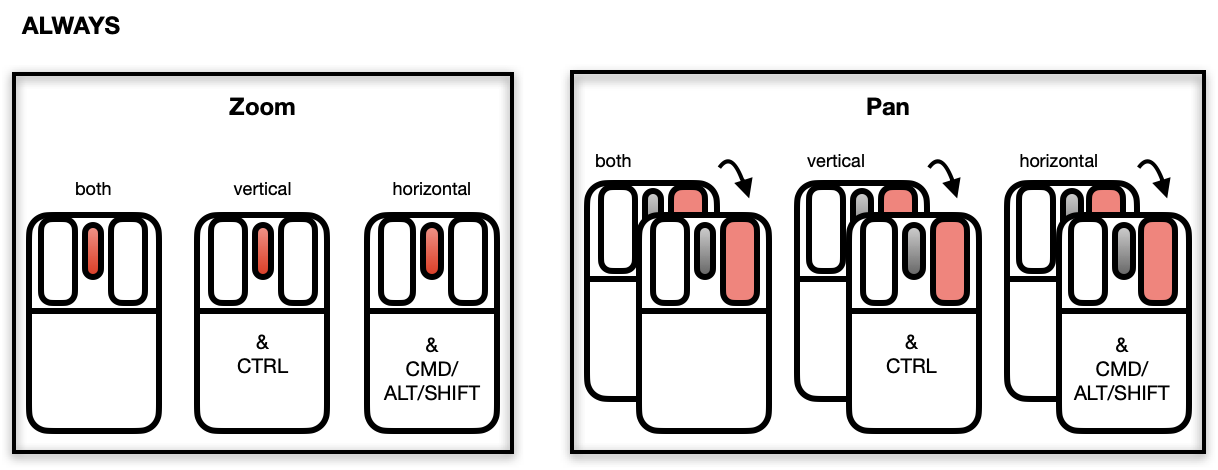
Selecting Points/Objects
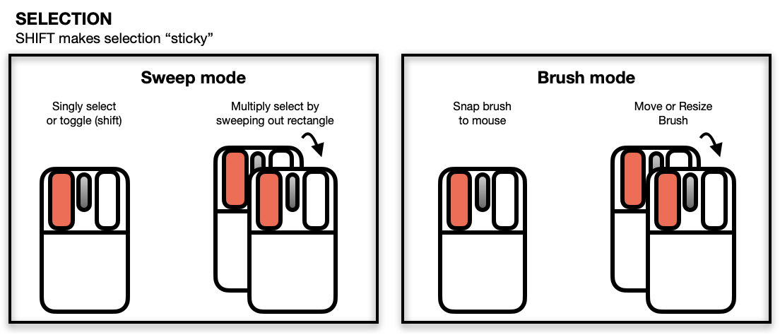
Moving Points on the Scatterplot Display
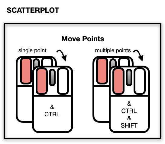
The scatterplot displays a number of direct interactions with the
mouse and keyboard, these include: zooming towards the mouse cursor using
the mouse wheel, panning by right-click dragging and various selection
methods using the left mouse button such as sweeping, brushing and
individual point selection. See the documentation for l_plot
for more details about the interaction gestures.
Some arguments to modify layouts can be passed through,
e.g. "separate", "ncol", "nrow", etc. Check l_facet
to see how these arguments work.
Value
-
The input is a
stlor adecomposed.tsobject, a structure of class"l_ts"containing four loon plots each representing a part of the decomposition by name: "original", "trend", "seasonal", and "remainder" -
The input is a vector, formula, data.frame, ...
by = NULL: aloonwidget will be returnedbyis notNULL: anl_facetobject (a list) will be returned and each element is aloonwidget displaying a subset of interest.
See Also
Turn interactive loon plot static loonGrob, grid.loon, plot.loon.
Density layer l_layer.density
Map layer l_layer, l_layer.map,
map
Other loon interactive states:
l_hist(),
l_info_states(),
l_serialaxes(),
l_state_names(),
names.loon()
Examples
if(interactive()) {
########################## l_plot.default ##########################
# default use as scatterplot

p1 <- with(iris, l_plot(Sepal.Length, Sepal.Width, color=Species,
                        title = "First plot"))

# The names of the info states that can be
# accessed or set.  They can also be given values as
# arguments to l_plot.default()
names(p1)
p1["size"] <- 10

p2 <- with(iris, l_plot(Petal.Length ~ Petal.Width,
                        linkingGroup="iris_data",
                        title = "Second plot",
                        showGuides = FALSE))
p2["showScales"] <- TRUE

# link first plot with the second plot requires
# l_configure to coordinate the synchroniztion
l_configure(p1, linkingGroup = "iris_data", sync = "push")

p1['selected'] <- iris$Species == "versicolor"
p2["glyph"][p1['selected']] <- "cdiamond"

gridExtra::grid.arrange(loonGrob(p1), loonGrob(p2), nrow = 1)

# Layout facets
### facet wrap
p3 <- with(mtcars, l_plot(wt, mpg, by = cyl, layout = "wrap"))
# it is equivalent to
# p3 <- l_plot(mpg~wt, by = ~cyl, layout = "wrap", on = mtcars)

### facet grid
p4 <- l_plot(x = 1:6, y = 1:6,
             by = size ~ color,
             size = c(rep(50, 2), rep(25, 2), rep(50, 2)),
             color = c(rep("red", 3), rep("green", 3)))

# Use with other tk widgets
tt <- tktoplevel()
tktitle(tt) <- "Loon plots with custom layout"

p1 <- l_plot(parent=tt, x=c(1,2,3), y=c(3,2,1))
p2 <- l_plot(parent=tt, x=c(4,3,1), y=c(6,8,4))

tkgrid(p1, row=0, column=0, sticky="nesw")
tkgrid(p2, row=0, column=1, sticky="nesw")

tkgrid.columnconfigure(tt, 0, weight=1)
tkgrid.columnconfigure(tt, 1, weight=1)

tkgrid.rowconfigure(tt, 0, weight=1)
########################## l_plot.decomposed.ts ##########################
decompose <- decompose(co2)
p <- l_plot(decompose, title = "Atmospheric carbon dioxide over Mauna Loa")
# names of plots in the display
names(p)
# names of states associated with the seasonality plot
names(p$seasonal)
# which can be set
p$seasonal['color'] <- "steelblue"

########################## l_plot.stl ##########################
co2_stl <- stl(co2, "per")
p <- l_plot(co2_stl, title = "Atmospheric carbon dioxide over Mauna Loa")
# names of plots in the display
names(p)
# names of states associated with the seasonality plot
names(p$seasonal)
# which can be set
p$seasonal['color'] <- "steelblue"
########################## l_plot.density ##########################
# plot a density estimate
set.seed(314159)
ds <- density(rnorm(1000))
p <- l_plot(ds,  title = "density estimate",
            xlabel = "x", ylabel = "density",
            showScales = TRUE)

########################## l_plot.map ##########################
if (requireNamespace("maps", quietly = TRUE)) {
   p <- l_plot(maps::map('world', fill=TRUE, plot=FALSE))
}
}
Create an interactive loon 3d plot widget
Description
l_plot3D is a generic function for creating interactive
visualization environments for R objects.
Usage
l_plot3D(x, y, z, ...)

## Default S3 method:
l_plot3D(
  x,
  y = NULL,
  z = NULL,
  axisScaleFactor = 1,
  by = NULL,
  on,
  layout = c("grid", "wrap", "separate"),
  connectedScales = c("cross", "row", "column", "both", "x", "y", "none"),
  color = l_getOption("color"),
  glyph = l_getOption("glyph"),
  size = l_getOption("size"),
  active = TRUE,
  selected = FALSE,
  xlabel,
  ylabel,
  zlabel,
  title,
  showLabels = TRUE,
  showScales = FALSE,
  showGuides = TRUE,
  guidelines = l_getOption("guidelines"),
  guidesBackground = l_getOption("guidesBackground"),
  foreground = l_getOption("foreground"),
  background = l_getOption("background"),
  parent = NULL,
  ...
)
Arguments
x |
the x, y and z arguments provide the x, y and z coordinates for the plot. Any reasonable way of defining the coordinates is acceptable. See the function xyz.coords for details. If supplied separately, they must be of the same length. |
y |
the y coordinates of points in the plot, optional if x is an appropriate structure. |
z |
the z coordinates of points in the plot, optional if x is an appropriate structure. |
... |
named arguments to modify plot states. |
axisScaleFactor |
the amount to scale the axes at the centre of the rotation. Default is 1. All numerical values are acceptable (0 removes the axes, < 0 inverts the direction of all axes.) |
by |
loon plot can be separated by some variables into multiple panels.
This argument can take a |
on |
if the |
layout |
layout facets as |
connectedScales |
Determines how the scales of the facets are to be connected depending
on which
|
color |
colours of points; colours are repeated
until matching the number points. Default is found using |
glyph |
the visual representation of the point. Argument values can be any of
|
size |
size of the symbol (roughly in terms of area).
Default is found using |
active |
a logical determining whether points appear or not
(default is |
selected |
a logical determining whether points appear selected at first
(default is |
xlabel |
Label for the horizontal (x) axis. If missing,
one will be inferred from |
ylabel |
Label for the vertical (y) axis. If missing,
one will be inferred from |
zlabel |
Label for the third (perpendicular to the screen) (z) axis. If missing,
one will be inferred from |
title |
Title for the plot, default is an empty string. |
showLabels |
logical to determine whether axes label (and title) should be presented. |
showScales |
logical to determine whether numerical scales should be presented on both axes. |
showGuides |
logical to determine whether to present background guidelines to help determine locations. |
guidelines |
colour of the guidelines shown when |
guidesBackground |
colour of the background to the guidelines shown when
|
foreground |
foreground colour used by all other drawing.
Default is found using |
background |
background colour used for the plot.
Default is found using |
parent |
a valid Tk parent widget path. When the parent widget is
specified (i.e. not |
Details
l_help() function call. The general direct manipulation and interaction gestures are outlined in the following figures.
Rotating
Press 'R' to toggle rotation mode. When rotation mode is active, either use the below mouse gestures or arrow keys to rotate the plot.
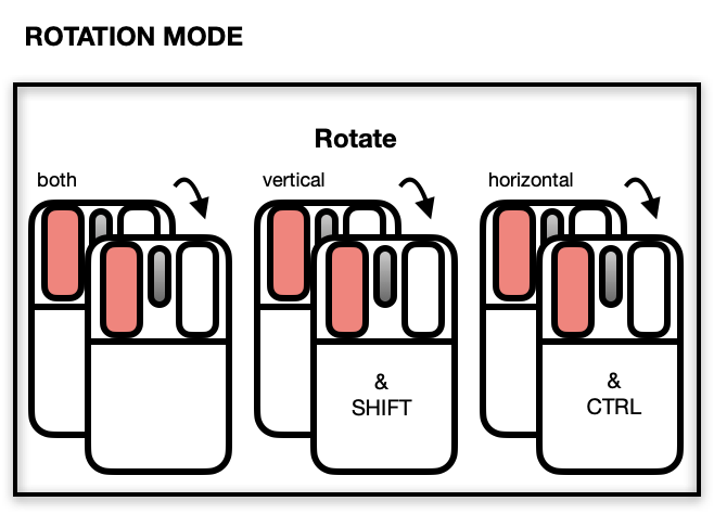
The centre of the rotation can be changed by panning the plot. To reset the rotation, use the tripod icon in the plot inspector.
Zooming and Panning
Selecting Points/Objects
Moving Points on the Scatterplot Display
NOTE: Although it is possible to programmatically add layers to an l_plot3D, these will not appear as part of the 3D plot's display. There is no provision at present to incorporate rotation of 3D geometric objects other than point glyphs.
The scatterplot displays a number of direct interactions with the
mouse and keyboard, these include: rotating, zooming towards the mouse cursor using
the mouse wheel, panning by right-click dragging and various selection
methods using the left mouse button such as sweeping, brushing and
individual point selection. See the documentation for l_plot3D
for more details about the interaction gestures.
Value
if the argument by is not set, a loon widget will be returned;
else an l_facet object (a list) will be returned and each element is
a loon widget displaying a subset of interest.
See Also
Turn interactive loon plot static loonGrob, grid.loon, plot.loon.
Other three-dimensional plotting functions:
l_scale3D()
Examples
if(interactive()){

with(quakes,
     l_plot3D(long, lat, depth, linkingGroup = "quakes")
)


with(l_scale3D(quakes),
     l_plot3D(long, lat, depth, linkingGroup = "quakes")
)

scaled_quakes <- l_scale3D(quakes)
with(scaled_quakes,
     l_plot3D(long, lat, depth, linkingGroup = "quakes")
)

with(scaled_quakes,
     l_plot3D(mag, stations, depth, linkingGroup = "quakes")
)

# Or together:
with(scaled_quakes,{
     l_plot3D(long, lat, depth, linkingGroup = "quakes")
     l_plot3D(mag, stations, depth, linkingGroup = "quakes")
     }
)

}
if(interactive()){

# default use as scatterplot

p1 <- with(quakes,
           l_plot3D(long, lat, depth)
           )

p2 <- with(quakes,
           l_plot3D(mag, stations, depth)
           )

# link the two plots p1 and p2
l_configure(p1, linkingGroup = "quakes", sync = "push")
l_configure(p2, linkingGroup = "quakes", sync = "push")

}
Arguments common to l_plot functions
Description
Like plot in R, l_plot is
the generic plotting function for objects in loon.
This is the workhorse of loon and is often a key part of many
other displays (e.g. l_pairs and l_navgraph)
Because plots in loon are interactive, the functions which create them
have many arguments in common. The value of these arguments become 'infostates' once the plot is instantiated. These can be accessed and set using the usual R square bracket operators '[]' and '[]<-' using the statename as a string. The state names can be found from an instantiated loon plot either via l_info_states() or, more in keeping with the R programming style, via names() (uses the method names.loon() for loon objects).
The same state names can be passed as arguments with values to a l_plot() call.
As arguments many of the common ones are desribed below.
Arguments
x |
the |
y |
argument description is as for the |
by |
loon plots can be separated by some variables into multiple panels. This argument can take a |
on |
if the |
layout |
layout facets as 'grid', 'wrap' or 'separate' |
connectedScales |
Determines how the scales of the facets are to be connected depending on which layout is used. |
linkingGroup |
a string naming a group of plots to be linked.
All plots with the same |
linkingKey |
an |
itemLabel |
an This action is commonly known as providing a "tool tip".
Note that all objects drawn in any layer of a plot (e.g. maps) will have an |
showItemLabels |
a logical (default |
color |
colours of points (default "grey60"); colours are repeated until matching the number points, |
glyph |
the visual representation of the point. Argument values can be any of
|
size |
size of the symbol (roughly in terms of area) |
active |
a logical determining whether points appear or not (default is TRUE for all points). If a logical vector is given of length equal to the number of points, then it identifies which points appear (TRUE) and which do not (FALSE). |
selected |
a logical determining whether points appear selected at first (default is FALSE for all points). If a logical vector is given of length equal to the number of points, then it identifies which points are (TRUE) and which are not (FALSE). |
xlabel |
Label for the horizontal (x) axis. If missing,
one will be inferred from |
ylabel |
Label for the vertical (y) axis. If missing,
one will be inferred from |
title |
Title for the plot, default is an empty string. |
minimumMargins |
the minimal size (in pixels) of the margins around the plot (bottom, left, top, right) |
showLabels |
logical to determine whether axes label (and title) should be presented. |
showScales |
logical to determine whether numerical scales should be presented on both axes. |
showGuides |
logical to determine whether to present background guidelines to help determine locations. |
guidelines |
colour of the guidelines shown when |
guidesBackground |
colour of the background to the guidelines shown when
|
foreground |
foreground colour used by all other drawing (default "black"). |
background |
background colour used for the plot (default "white") |
parent |
a valid Tk parent widget path. When the parent widget is
specified (i.e. not |
... |
named arguments to modify plot states. |
Details
The interactive displays permit a number of direct interactions using the
mouse and keyboard, these include: zooming towards the mouse cursor using
the mouse wheel, panning by right-click dragging and various selection
methods using the left mouse button such as sweeping, brushing and
individual point selection. See the documentation for l_plot
for more details about the interaction gestures.
See Also
the demos demo(l_glyph_sizes, package = "loon"), demo(l_glyphs, package = "loon"),
and demo(l_make_glyphs, package = "loon").
Examples
   ## Not run:
    # default use as scatterplot

    p1 <- with(iris, l_plot(x = Sepal.Length,
                            y = Sepal.Width,
                            color=Species,
                            title = "Sepal sizes"))

    # The names of the info states that can be
    # accessed or set.  They can also be given values as
    # arguments to l_plot.default()
    names(p1)
    versicolor <- (iris$Species == "versicolor")
    p1["size"] <- 10
    p1["glyph"][versicolor]<- "csquare"
    p1["minimumMargins"][1] <- 100

## End(Not run)
Create a Scatterplot Inspector
Description
Inpectors provide graphical user interfaces to oversee and modify plot states
Usage
l_plot_inspector(parent = NULL, ...)
Arguments
parent |
parent widget path |
... |
state arguments |
Value
widget handle
See Also
Examples
if(interactive()){

i <- l_plot_inspector()
}
Create a Scatterplot Analysis Inspector
Description
Inpectors provide graphical user interfaces to oversee and modify plot states
Usage
l_plot_inspector_analysis(parent = NULL, ...)
Arguments
parent |
parent widget path |
... |
state arguments |
Value
widget handle
See Also
Examples
if(interactive()){

i <- l_plot_inspector_analysis()
}
Draw a decomposed time series loon plot
Description
l_plot_ts is a generic function for creating a decomposed time series plot. It
is mainly used in l_plot.decomposed.ts and l_plot.stl
Usage
l_plot_ts(
  x,
  color = l_getOption("color"),
  size = l_getOption("size"),
  linecolor = l_getOption("color"),
  linewidth = l_getOption("linewidth"),
  xlabel = NULL,
  ylabel = NULL,
  title = NULL,
  tk_title = NULL,
  linkingGroup,
  showScales = TRUE,
  showGuides = TRUE,
  showLabels = TRUE,
  call = match.call(),
  ...
)
Arguments
x |
Either an |
color |
points colour of all time series.
Default is given by |
size |
points size of all time series.
Default is given by |
linecolor |
line colour of all time series.
Default is given by |
linewidth |
line width of all time series (incl. original and decomposed components.
Default is given by |
xlabel |
the labels for the x axes. This is a length four character vector one for each: of the original
time series, the trend component, the seasonality component, and the remainder. If of length 1, the label is repeated; if |
ylabel |
the labels for the vertical axes. This is a length four character vector one for each: of the original
time series, the trend component, the seasonality component, and the remainder. If |
title |
an overall title for the entire display. If |
tk_title |
provides an alternative window name to Tk's |
linkingGroup |
name of linking group.
If missing, one is created from the data name and class associated with |
showScales |
a logical as to whether to display the scales on all axes, default is TRUE. |
showGuides |
a logical as to whether to display background guide lines on all plots, default is TRUE. |
showLabels |
a logical as to whether to display axes labels on all plots, default is TRUE. |
call |
a call in which all of the specified arguments are specified by their full names |
... |
keyword value pairs passed off to |
Value
A structure of class "l_ts" containing four loon plots each representing a part of the decomposition
by name: "original", "trend", "seasonal", and "remainder".
See Also
l_plot.stl, l_plot.decomposed.ts,
stl, or decompose.
Model Prediction
Description
It is entirely for the purpose of plotting fits and intervals on a scatterplot (or histogram).
It is a generic function to predict models for loon smooth layer (a wrap of the function predict).
However, the output is unified.
Usage
l_predict(model, ...)

## Default S3 method:
l_predict(model, ...)

## S3 method for class 'lm'
l_predict(
  model,
  newdata = NULL,
  interval = c("none", "confidence", "prediction"),
  level = 0.95,
  ...
)

## S3 method for class 'nls'
l_predict(
  model,
  newdata = NULL,
  interval = c("none", "confidence", "prediction"),
  level = 0.95,
  ...
)

## S3 method for class 'glm'
l_predict(
  model,
  newdata = NULL,
  interval = c("none", "confidence"),
  level = 0.95,
  ...
)

## S3 method for class 'loess'
l_predict(
  model,
  newdata = NULL,
  interval = c("none", "confidence", "prediction"),
  level = 0.95,
  ...
)
Arguments
model |
a model object for which prediction is desired |
... |
arguments passed in |
newdata |
optionally, a data frame in which to look for variables with which to predict. If omitted, the fitted linear predictors are used. |
interval |
type of interval, could be "none", "confidence" or "prediction" (not for |
level |
confidence level |
Value
A data frame is returned with x (if newdata is given) and y.
If the interval is not none,
two more columns, lower (lower interval) and upper (upper interval) will be returned.
Examples
y <- rnorm(10)
x <- rnorm(10)
model1 <- lm(y ~ x)
# formal output
pre <- l_predict(model1, newdata = data.frame(x = sort(x)),
                 interval = "conf")
head(pre)

if(interactive()) {
p <- with(cars, l_plot(speed, dist))

# Example taken from
# https://stackoverflow.com/questions/23852505/how-to-get-confidence-interval-for-smooth-spline
#
l_predict.smooth.spline <- function(model, interval = c("confidence", "none"),
                                    level = 0.95, ...) {
# confidence interval of `smooth.spline`
  interval <- match.arg(interval)

  res <- (model$yin - model$y)/(1 - model$lev)     # jackknife residuals
  sigma <- sqrt(var(res))                          # estimate sd
  std <- stats::qnorm(level / 2 + 0.5)
  upper <- model$y + std * sigma * sqrt(model$lev) # upper 95% conf. band
  lower <- model$y - std * sigma * sqrt(model$lev) # lower 95% conf. band

  data.frame(y = model$yin, lower = lower, upper = upper)
}
l <- l_layer_smooth(p, method = "smooth.spline", interval = "confidence")
}
The primitive glyphs available to a scatterplot or graph display
Description
Returns a vector of the available primitive glyphs.
Usage
l_primitiveGlyphs()
Details
The scatterplot and graph displays both have the n-dimensional state
'glyph' that assigns each data point or graph node a glyph (i.e. a
visual representation).
Loon distinguishes between primitive and non-primitive glyphs: the primitive glyphs are always available for use whereas the non-primitive glyphs need to be first specified and added to a plot before they can be used.
The primitive glyphs are:
For more information run: l_help("learn_R_display_plot.html#glyphs")
Value
A character vector of the names of all primitive glyphs in loon.
See Also
Other glyph functions:
l_glyph_add(),
l_glyph_add.default(),
l_glyph_add_image(),
l_glyph_add_pointrange(),
l_glyph_add_polygon(),
l_glyph_add_serialaxes(),
l_glyph_add_text(),
l_glyph_delete(),
l_glyph_getLabel(),
l_glyph_getType(),
l_glyph_ids(),
l_glyph_relabel()
Force a Content Redraw of a Plot
Description
Force redraw the plot to make sure that all the visual elements are placed correctly.
Usage
l_redraw(widget)
Arguments
widget |
widget path as a string or as an object handle |
Details
Note that this function is intended for debugging. If you find that the display does not display the data according to its plot states then please contact loon's package maintainer.
Examples
if(interactive()){

p <- l_plot(iris)
l_redraw(p)

}
Resize Plot Widget
Description
Resizes the toplevel widget to a specific size.
Usage
l_resize(widget, width, height)
Arguments
widget |
widget path as a string or as an object handle |
width |
width in pixels |
height |
in pixels |
See Also
Examples
if(interactive()){

p <- l_plot(iris)

l_resize(p, 300, 300)
l_size(p) <- c(500, 500)

}
Save the info states of a loon plot widget in a file
Description
l_saveStates uses saveRDS()
to save the info states of a loon plot as an R object to the named file.
This is helpful, for example, when using RMarkdown or some other notebooking
facility to recreate an earlier saved loon plot so as to present it
in the document.
Usage
l_saveStates(
  p,
  states = c("color", "active", "selected", "linkingKey", "linkingGroup"),
  file = stop("missing name of file"),
  ...
)
Arguments
p |
the 'l_plot' object whose info states are to be saved. |
states |
either the logical 'TRUE' or a character vector of info states to be saved. Default value 'c("color", "active", "selected", "linkingKey", "linkingGroup")' consists of 'n' dimensional states that are common to many 'l_plot's and which are most important to reconstruct the plot's display in any summary. If 'states' is the logical 'TRUE', by 'names(p)' are saved. |
file |
is a string giving the file name where the saved information' will be written (custom suggests this file name end in the suffix '.rds'. |
... |
further arguments passed to |
Value
a list of class 'l_savedStates' containing the states and their values. Also has an attribute 'l_plot_class' which contains the class vector of the plot 'p'
See Also
l_getSavedStates l_copyStates l_info_states readRDS saveRDS
Examples
if(interactive()){
#
# Suppose you have some plot that you created like
p <- l_plot(iris, showGuides = TRUE)
#
# and coloured groups by hand (using the mouse and inspector)
# so that you ended up with these colours:
p["color"] <- rep(c( "lightgreen", "firebrick","skyblue"),
                  each = 50)
#
# Having determined the colours you could save them (and other states)
# in a file of your choice, here some tempfile:
myFileName <- tempfile("myPlot", fileext = ".rds")
#
# Save the named states of p
l_saveStates(p,
             states = c("color", "active", "selected"),
             file = myFileName)
#
# These can later be retrieved and used on a new plot
# (say in RMarkdown) to set the new plot's values to those
# previously determined interactively.
p_new <- l_plot(iris, showGuides = TRUE)
p_saved_info <- l_getSavedStates(myFileName)
#
# We can tell what kind of plot was saved
attr(p_saved_info, "l_plot_class")
#
# The result is a list of class "l_savedStates" which
# contains the names of the
p_new["color"] <- p_saved_info$color
#
# The result is that p_new looks like p did
# (after your interactive exploration)
# and can now be plotted as part of the document
plot(p_new)
#
# For compound plots, the info_states are saved for each plot
pp <- l_pairs(iris)
myPairsFile <- tempfile("myPairsPlot", fileext = ".rds")
#
# Save the names states of pp
l_saveStates(pp,
             states = c("color", "active", "selected"),
             file = myPairsFile)
pairs_info <-  l_getSavedStates(myPairsFile)
#
# For compound plots, the info states for all constitutent
# plots are saved.  The result is a list of class "l_savedStates"
# whose elements are the named plots as "l_savedStates"
# themselves.
#
# The names of the plots which were saved
names(pairs_info)
#
# And the names of the info states whose values were saved for
# the first plot
names(pairs_info$x2y1)
#
# While it is generally recommended to access (or assign) saved
# state values using the $ sign accessor, paying attention to the
# nested list structure of an "l_savedStates" object (especially for
# l_compound plots), R's square bracket notation [] has also been
# specialized to allow a syntactically simpler (but less precise)
# access to the contents of an l_savedStates object.
#
# For example,
p_saved_info["color"]
#
# returns the saved "color" as a vector of colours.
#
# In contrast,
pairs_info["x2y1"]
# returns the l_savedStates object of the states of the plot named "x2y1",
# but
pairs_info["color"]
# returns a LIST of colour vectors, by plot as they were named in pairs_info
#
# As a consequence, the following two are equivalent,
pairs_info["x2y1"]["color"]
# finds the value of "color" from an "l_savedStates" object
# whereas
pairs_info["color"][["x2y1"]]
# finds the value of "x2y1" from a "list" object
#
# Also, setting a state of an "l_savedStates" is possible
# (though not generally recommended; better to save the states again)
#
p_saved_info["color"] <- rep("red", 150)
# changes the saved state "color" on p_saved_info
# whereas
pairs_info["color"] <- rep("red", 150)
# will set the red color for any plot within pairs_info having "color" saved.
# In this way the assignment function via [] is trying to be clever
# for l_savedStates for compound plots and so may have unintentional
# consequences if the user is not careful.

# Generally, one does not want/need to change the value of saved states.
# Instead, the states would be saved again from the interactive plot
# if change is necessary.
# Alternatively, more nuanced and careful control is maintained using
# the $ selectors for lists.
}
Scale for 3d plotting
Description
l_scale3D scales its argument in a variety of ways
used for 3D visualization.
Usage
l_scale3D(x, center = TRUE, method = c("box", "sphere"))
Arguments
x |
the matrix or data.frame whose columns are to be scaled.
Any |
center |
either a logical value or numeric-alike vector of length equal
to the number of columns of |
method |
the scaling method to use.
If |
Value
a data.frame whose columns are centred and scaled according to
the given arguments. For method = "sphere"), the three variable names are
x1, x2, and x3.
See Also
Other three-dimensional plotting functions:
l_plot3D()
Examples
##### Iris data
#
# All variables (including Species as a factor)
result_box <- l_scale3D(iris)
head(result_box, n = 3)
apply(result_box, 2, FUN = range)
# Note mean is not zero.
apply(result_box, 2, FUN = mean)


# Sphering only on 3D data.
result_sphere <- l_scale3D(iris[, 1:3], method = "sphere")
head(result_sphere, n = 3)
apply(result_sphere, 2, FUN = range)
# Note mean is numerically zero.
apply(result_sphere, 2, FUN = mean)


#  With NAs
x <- iris
x[c(1, 3), 1] <- NA
x[2, 3] <- NA

result_box <- l_scale3D(x)
head(result_box, n = 5)
apply(result_box, 2, FUN = function(x) {range(x, na.rm = TRUE)})

# Sphering only on 3D data.
result_sphere <- l_scale3D(x[, 1:3], method = "sphere")
# Rows having had any NA are all NA after sphering.
head(result_sphere, n = 5)
# Note with NAs mean is no longer numerically zero.
# because centring was based on all non-NAs in each column
apply(result_sphere, 2, FUN = function(x) {mean(x, na.rm = TRUE)})
Change Plot Region to Display All Active Data
Description
The function modifies the zoomX, zoomY,
panX, and panY so that all active data points are displayed.
Usage
l_scaleto_active(widget)
Arguments
widget |
widget path as a string or as an object handle |
Change Plot Region to Display All Elements of a Particular Layer
Description
The function modifies the zoomX, zoomY,
panX, and panY so that all elements of a particular layer are
displayed.
Usage
l_scaleto_layer(target, layer)
Arguments
target |
either an object of class loon or a vector that specifies the
widget, layer, glyph, navigator or context completely. The widget is
specified by the widget path name (e.g. |
layer |
layer id |
See Also
Change Plot Region to Display the All Data of the Model Layer
Description
The function modifies the zoomX, zoomY,
panX, and panY so that all elements in the model layer of the
plot are displayed.
Usage
l_scaleto_plot(widget)
Arguments
widget |
widget path as a string or as an object handle |
Change Plot Region to Display All Selected Data
Description
The function modifies the zoomX, zoomY,
panX, and panY so that all selected data points are
displayed.
Usage
l_scaleto_selected(widget)
Arguments
widget |
widget path as a string or as an object handle |
Change Plot Region to Display All Plot Data
Description
The function modifies the zoomX, zoomY,
panX, and panY so that all elements in the plot are
displayed.
Usage
l_scaleto_world(widget)
Arguments
widget |
widget path as a string or as an object handle |
Create an interactive serialaxes (parallel axes or radial axes) plot
Description
l_serialaxes is a generic function for displaying multivariate data either as a
stacked star glyph plot, or as a parallel coordinate plot.
Usage
l_serialaxes(data, ...)

## Default S3 method:
l_serialaxes(
  data,
  sequence,
  scaling = "variable",
  axesLayout = "radial",
  by = NULL,
  on,
  layout = c("grid", "wrap", "separate"),
  andrews = FALSE,
  showAxes = TRUE,
  color = l_getOption("color"),
  active = TRUE,
  selected = FALSE,
  linewidth = l_getOption("linewidth"),
  parent = NULL,
  ...
)
Arguments
data |
a data frame with numerical data only |
... |
named arguments to modify the serialaxes states or layouts, see details. |
sequence |
vector with variable names that defines the axes sequence |
scaling |
one of 'variable', 'data', 'observation' or 'none' to specify how the data is scaled. See Details and Examples for more information. |
axesLayout |
either |
by |
loon plot can be separated by some variables into multiple panels.
This argument can take a |
on |
if the |
layout |
layout facets as |
andrews |
Andrew's plot (a 'Fourier' transformation) |
showAxes |
boolean to indicate whether axes should be shown or not |
color |
vector with line colors. Default is given by |
active |
a logical determining whether points appear or not
(default is |
selected |
a logical determining whether points appear selected at first
(default is |
linewidth |
vector with line widths. Default is given by |
parent |
a valid Tk parent widget path. When the parent widget is
specified (i.e. not |
Details
For more information run: l_help("learn_R_display_hist")
-
The
scalingstate defines how the data is scaled. The axes display 0 at one end and 1 at the other. For the following explanation assume that the data is in a nxp dimensional matrix. The scaling options are thenvariable per column scaling observation per row scaling data whole matrix scaling none do not scale -
Some arguments to modify layouts can be passed through, e.g. "separate", "byrow", etc. Check
l_facetto see how these arguments work.
Value
if the argument by is not set, a loon widget will be returned;
else an l_facet object (a list) will be returned and each element is
a loon widget displaying a subset of interest.
See Also
Turn interactive loon plot static loonGrob, grid.loon, plot.loon.
Other loon interactive states:
l_hist(),
l_info_states(),
l_plot(),
l_state_names(),
names.loon()
Examples
if(interactive()){

#######
#
# Effect of the choice of the argument "scaling"
#
# To illustrate we will look at the four measurements of
# 150 iris flowers from the iris data of Edgar Anderson made
# famous by R.A. Fisher.
#
# First separate the measurements
irisFlowers <- iris[, 1:4]
# from their species
species <- iris[,5]
# and get some identifiers for the individual flowers
flowerIDs <- paste(species, 1:50)
#
# Now create parallel axes plots of the measurements
# using different scaling values.

#
# scaling = "variable"
#
# This is the standard scaling of most serial axes plots,
# scaling each axis from the minimum to the maximum of that variable.
# Hence it is the default scaling.
#
# More precisely, it maps the minimum value in each column (variable) to
# zero and the maximum to one.  The result is every parallel
# axis will have a point at 0 and a point at 1.
#
# This scaling highlights the relationships (e.g. correlations)
# between the variables (removes the effect of the location and scale of
# each variable).
#
# For the iris data, ignoring species we see for example that
# Sepal.Length and Sepal.Width are negatively correlated (lots of
# crossings) across species but more positively correlated (mostly
# parallel lines) within each species (colour).
#
sa_var <- l_serialaxes(irisFlowers,
                       scaling = "variable",    # scale within column
                       axesLayout = "parallel",
                       color = species,
                       linewidth = 2,
                       itemLabel = flowerIDs,
                       showItemLabels = TRUE,
                       title = "scaling = variable (initially)",
                       linkingGroup = "irisFlowers data")

#
# scaling = "observation"
#
# This maps the minimum value in each row (observation) to
# zero and the maximum value in each row to one.
#
# The result is that every observation (curve in the parallel
# coordinate plot) will touch 0 on at least one axis and touch
# 1 on another.
#
# This scaling highlights the differences between observations (rows)
# in terms of the relative measurements across the variables for each
# observation.
#
# For example, for the iris data we can see that for every flower (row)
# the Sepal.Length is the largest measurement and the Petal.Width
# is the smallest.  Each curve gives some sense of the *shape* of each
# flower without regard to its size.  Two species (versicolor and
# virginica) have similar shaped flowers (relatively long but narrow
# sepals and petals), whereas the third (setosa) has relatively large
# sepals compared to small petals.
#
sa_obs <- l_serialaxes(irisFlowers,
                       scaling = "observation", # scale within row
                       axesLayout = "parallel",
                       color = species,
                       linewidth = 2,
                       itemLabel = flowerIDs,
                       showItemLabels = TRUE,
                       title = "scaling = observation (initially)",
                       linkingGroup = "irisFlowers data")

#
# scaling = "data"
#
# This maps the minimum value in the whole dataset (over all elements)
# to zero and the maximum value in the whole dataset to one.
#
# The result is that every measurement is on the same numeric (if not
# measurement) scale.  Highlighting the relative magnitudes of all
# numerical values in the data set, each curve shows the relative magnitudes
# without rescaling by variable.
#
# This is most sensible data such as the iris flower where all four measurements
# appear to have been taken on the same measuring scale.
#
# For example, for the iris data full data scaling preserves the size
# and shape of each flower.  Again virginica is of roughly the same
# shape as versicolor but has distinctly larger petals.
# Setosa in contrast is quite differently shaped in both sepals and petals
# but with sepals more similar in size to the two other flowers and
# with significantly smaller petals.
sa_dat <- l_serialaxes(irisFlowers,
                       scaling = "data",        # scale using all data
                       axesLayout = "parallel",
                       color = species,
                       linewidth = 2,
                       itemLabel = flowerIDs,
                       showItemLabels = TRUE,
                       title = "scaling = data (initially)",
                       linkingGroup = "irisFlowers data")

#
#  scaling = "none"
#
#  Sometimes we might wish to choose a min and max to use
#  for the whole data set; or perhaps a separate min and max
#  for each variable.

#  This would be done outside of the construction of the plot
#  and displayed by having scaling = "none" in the plot.
#
#  For example, for the iris data, we might choose scales so that
#  the minimum and the maximum values within the data set do not
#  appear at the end points 0 and 1 of the axes but instead inside.
#
#  Suppose we choose the following limits for all variables
lower_lim <- -3 ; upper_lim <- max(irisFlowers) + 1

#  These are the limits we want to use to define the end points of
#  the axes for all variables.
#  We need only scale the data as
irisFlowers_0_1 <- (irisFlowers - lower_lim)/(upper_lim - lower_lim)
#  Or alternatively using the built-in scale function
#  (which allows different scaling for each variable)
irisFlowers_0_1 <- scale(irisFlowers,
                         center = rep(lower_lim, 4),
                         scale = rep((upper_lim - lower_lim), 4))

# Different scales for different
# And instruct the plot to not scale the data but plot it on the 0-1 scale
# for all axes.  (Note any rescaled date outside of [0,1] will not appear.)
#
sa_none <- l_serialaxes(irisFlowers_0_1,
                        scaling = "none",        # do not scale
                        axesLayout = "parallel",
                        color = species,
                        linewidth = 2,
                        itemLabel = flowerIDs,
                        showItemLabels = TRUE,
                        title = "scaling = none (initially)",
                        linkingGroup = "irisFlowers data")

# This is particularly useful for "radial" axes to keep the polygons away from
# the centre of the display.
# For example
sa_none["axesLayout"] <- "radial"
# now displays each flower as a polygon where shapes and sizes are easily
# compared.
#
#  NOTE: rescaling the data so that all values are within [0,1] is perhaps
#        the best way to proceed (especially if there are natural lower and
#        upper limits for each variable).
#        Then scaling can always be changed via the inspector.

}
Create a Serialaxes Inspector
Description
Inpectors provide graphical user interfaces to oversee and modify plot states
Usage
l_serialaxes_inspector(parent = NULL, ...)
Arguments
parent |
parent widget path |
... |
state arguments |
Value
widget handle
See Also
Examples
if(interactive()){

i <- l_serialaxes_inspector()
}
Set the aspect ratio of a plot
Description
The aspect ratio is defined by the ratio of the number of pixels for one data unit on the y axis and the number of pixels for one data unit on the x axes.
Usage
l_setAspect(widget, aspect, x, y)
Arguments
widget |
widget path as a string or as an object handle |
aspect |
aspect ratio, optional, if omitted then the |
x |
optional, if the |
y |
see description for |
Examples
## Not run:
p <- with(iris, l_plot(Sepal.Length ~ Sepal.Width, color=Species))

l_aspect(p)
l_setAspect(p, x = 1, y = 2)

## End(Not run)
Use custom colors for mapping nominal values to distinct colors
Description
Modify loon's color mapping list to a set of custom colors.
Usage
l_setColorList(colors)
Arguments
colors |
vector with valid color names or hex-encoded colors |
Details
There are two commonly used mapping schemes of data values to colors: one scheme maps numeric values to colors on a color gradient and the other maps nominal data to colors that can be well differentiated visually (e.g. to highlight the different groups). Presently, loon always uses the latter approach for its color mappings. You can use specialized color pallettes to map continuous values to color gradients as shown in the examples below.
When assigning values to a display state of type color then loon maps those values using the following rules
if all values already represent valid Tk colors (see
tkcolors) then those colors are taken.if the number of distinct values are less than number of values in loon's color mapping list then they get mapped according to the color list, see
l_setColorListandl_getColorList.if there are more distinct values as there are colors in loon's color mapping list then loon's own color mapping algorithm is used. See
loon_paletteand for more details about the algorithm below in this documentation.
Loon's default color list is composed of the first 11 colors from the hcl color wheel (displayed below in the html version of the documentation). The letters in hcl stand for hue, chroma and luminance, and the hcl wheel is useful for finding "balanced colors" with the same chroma (radius) and luminance but with different hues (angles), see Ross Ihaka (2003) "Colour for presentation graphics", Proceedings of DSC, p. 2 (https://www.stat.auckland.ac.nz/~ihaka/courses/787/color.pdf).
The colors in loon's internal color list are also the default ones listed
as the "modify color actions" in the analysis inspectors. To query and
modify loon's color list use l_getColorList and
l_setColorList.
In the case where there are more unique data values than colors in loon's color list then the colors for the mapping are taken from different locations distributed on the hcl color wheel (see above).
One of the advantages of using the hcl color wheel is that one can obtain any number of "balanced colors" with distinct hues. This is useful in encoding data with colors for a large number of groups; however, it should be noted that the more groups we have the closer the colors sampled from the wheel become and, therefore, the more similar in appearance.
A common way to sample distinct "balanced colors" on the hcl wheel is to
choose evenly spaced hues distributed on the wheel (i.e. angles on the
wheel). However, this approach leads to color sets where most colors change
when the sample size (i.e. the number of sampled colors from the wheel)
increases by one. For loon, it is desirable to have the first m
colors of a color sample of size m+1 to be the same as the colors in
a color sample of size m, for all positive natural numbers m.
Hence, we prefer to have a sequence of colors. This way, the colors on the
inspectors stay relevant (i.e. they match with the colors of the data
points) when creating plots that encode with color a data variable with
different number of groups.
We implemented such a color sampling scheme (or color sequence generator)
that also makes sure that neighboring colors in the sequence have different
hues. In you can access this color sequence generator with
loon_palette. The color wheels below show the color
generating sequence twice, once for 16 colors and once for 32 colors.
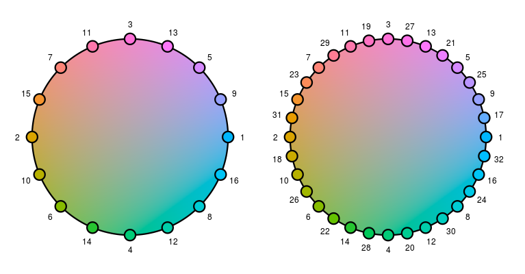
Note, for the inspector: If there are more unique colors in the data points than there are on the inspectors then it is possible to add the next five colors in the sequence of the colors with the +5 button. Alternatively, the + button on the modify color part of the analysis inspectors allows the user to pick any additional color with a color menu. Also, if you change the color mapping list and close and re-open the loon inspector these new colors show up in the modify color list.
When other color mappings of data values are required (e.g. numerical data
to a color gradient) then the functions in the scales
R package provide various mappings including mappings for qualitative,
diverging and sequential values.
See Also
l_setColorList, l_getColorList,
l_setColorList_ColorBrewer, l_setColorList_hcl,
l_setColorList_baseR
Examples
if(interactive()){


l_plot(1:3, color=1:3) # loon's default mapping

cols <- l_getColorList()
l_setColorList(c("red", "blue", "green", "orange"))

## close and reopen inspector

l_plot(1:3, color=1:3)   # use the new color mapping
l_plot(1:10, color=1:10) # use loons default color mapping as color list is too small

# reset to default
l_setColorList(cols)
}

## Not run:
# you can also perform the color mapping yourself, for example with
# the col_numeric function provided in the scales package
if (requireNamespace("scales", quietly = TRUE)) {
  p_custom <- with(olive, l_plot(stearic ~ oleic,
       color = scales::col_numeric("Greens", domain = NULL)(palmitic)))
  }

## End(Not run)
Set loon's color mapping list to the colors from ColorBrewer
Description
Loon's color list is used to map nominal values to colors. See
the documentation for l_setColorList.
Usage
l_setColorList_ColorBrewer(
  palette = c("Set1", "Set2", "Set3", "Pastel1", "Pastel2", "Paired", "Dark2", "Accent")
)
Arguments
palette |
one of the following RColorBrewer palette name: Set1, Set2, Set3, Pastel1, Pastel2, Paired, Dark2, or Accent |
Details
Only the following palettes in ColorBrewer are available: Set1, Set2, Set3, Pastel1, Pastel2, Paired, Dark2, and Accent. See the examples below.
See Also
l_setColorList, l_setColorList_loon,
l_setColorList_ColorBrewer, l_setColorList_hcl,
l_setColorList_baseR, l_setColorList_ggplot2
Examples
if (interactive()){

## Not run:
if (requireNamespace("RColorBrewer", quietly = TRUE)) {
  RColorBrewer::display.brewer.all()
}

## End(Not run)

l_setColorList_ColorBrewer("Set1")
p <- l_plot(iris)

}
Set loon's color mapping list to the colors from base R
Description
Loon's color list is used to map nominal values to colors. See
the documentation for l_setColorList.
Usage
l_setColorList_baseR()
See Also
l_setColorList, l_setColorList_loon,
l_setColorList_ColorBrewer, l_setColorList_hcl,
l_setColorList_baseR, l_setColorList_ggplot2
Set loon's color mapping list to the colors from ggplot2
Description
Loon's color list is used to map nominal values to colors. See
the documentation for l_setColorList.
Usage
l_setColorList_ggplot2()
See Also
l_setColorList, l_setColorList_loon,
l_setColorList_ColorBrewer, l_setColorList_hcl,
l_setColorList_baseR, l_setColorList_ggplot2
Set loon's color mapping list to the colors from hcl color wheen
Description
Loon's color list is used to map nominal values to colors. See
the documentation for l_setColorList.
Usage
l_setColorList_hcl(chroma = 56, luminance = 51, hue_start = 231)
Arguments
chroma |
The chroma of the color. The upper bound for chroma depends on hue and luminance. |
luminance |
A value in the range [0,100] giving the luminance of the colour. For a given combination of hue and chroma, only a subset of this range is possible. |
hue_start |
The start hue for sampling. The hue of the color specified as an angle in the range [0,360]. 0 yields red, 120 yields green 240 yields blue, etc. |
Details
Samples equally distant colors from the hcl color wheel. See the
documentation for hcl for more information.
See Also
l_setColorList, l_setColorList_loon,
l_setColorList_ColorBrewer, l_setColorList_hcl,
l_setColorList_baseR, l_setColorList_ggplot2
Set loon's color mapping list to the colors from loon defaults
Description
Loon's color list is used to map nominal values to colors. See
the documentation for l_setColorList.
Usage
l_setColorList_loon()
See Also
l_setColorList, l_setColorList_loon,
l_setColorList_ColorBrewer, l_setColorList_hcl,
l_setColorList_baseR, l_setColorList_ggplot2
Modify States of a Plot that are Linked in Loon's Standard Linking Model
Description
Loon's standard linking model is based on three levels, the
linkingGroup and linkingKey states and the used
linkable states. See the details below.
Usage
l_setLinkedStates(widget, states)
Arguments
widget |
widget path as a string or as an object handle |
states |
used linkable state names, see in details below |
Details
Loon's standard linking model is based on two states,
linkingGroup and linkingKey. The full capabilities of the
standard linking model are described here. However, setting the
linkingGroup states for two or more displays to the same string is
generally all that is needed for linking displays that plot data from the
same data frame. Changing the linking group of a display is also the only
linking-related action available on the analysis inspectors.
The first linking level is as follows: loon's displays are linked if they
share the same string in their linkingGroup state. The default
linking group 'none' is a keyword and leaves a display un-linked.
The second linking level is as follows. All n-dimensional states can
be linked between displays. We call these states linkable. Further,
only linkable states with the same name can be linked between displays. One
consequence of this shared state name rule is that, with the
standard linking model, the linewidth state of a serialaxes display
cannot be linked with the size state of a scatterplot display. Also,
each display maintains a list that defines which of its linkable states
should be used for linking; we call these states the used linkable
states. The default used linkable states are as follows
| Display | Default used linkable states |
| scatterplot | selected, color, active,
size |
| histogram | selected, color,
active |
| serialaxes | selected, color, active |
| graph | selected, color, active, size
|
If any two displays are set to be linked (i.e. they share the same linking group) then the intersection of their used linkable states are actually linked.
The third linking level is as follows. Every display has a
n-dimensional linkingKey state. Hence, every data point has
an associated linking key. Data points between linked plots are linked if
they share the same linking key.
Set the value of a loon display option
Description
All of loon's displays access a set of common options. This function assigns the value to the named option.
Usage
l_setOption(option, value)
Arguments
option |
the name of the option being set |
value |
the value to be assigned to the option. If value == "default", then the option is set to loon's default value for it. |
Value
the new value
See Also
l_getOption, l_getOptionNames, l_userOptions,
l_userOptionDefault
Examples
l_setOption("select-color", "red")
l_setOption("select-color", "default")
Set the title font of all loon displays
Description
All of loon's displays access a set of common options. This function sets the font for the title bar of the displays.
Usage
l_setTitleFont(size = "16", weight = "bold", family = "Helvetica")
Arguments
size |
the font size. |
weight |
the font size. |
family |
the font family. |
Value
the value of the named option.
See Also
l_getOptionNames, l_userOptions,
l_userOptionDefault, l_setOption
Query Size of a Plot Display
Description
Get the width and height of a plot in pixels
Usage
l_size(widget)
Arguments
widget |
widget path as a string or as an object handle |
Value
Vector width width and height in pixels
See Also
Resize Plot Widget
Description
Resizes the toplevel widget to a specific size. This setter
function uses l_resize.
Usage
l_size(widget) <- value
Arguments
widget |
widget path as a string or as an object handle |
value |
numeric vector of length 2 with width and height in pixels |
See Also
Examples
if(interactive()){

p <- l_plot(iris)

l_resize(p, 300, 300)
l_size(p) <- c(500, 500)

}
Get State Names of Loon Object
Description
States of loon objects can be accessed `[` and l_cget
and modified with l_configure.
Usage
l_state_names(target)
Arguments
target |
either an object of class loon or a vector that specifies the
widget, layer, glyph, navigator or context completely. The widget is
specified by the widget path name (e.g. |
Details
In order to access values of a states use l_info_states.
Value
state names
See Also
l_info_states, l_cget, l_configure
Other loon interactive states:
l_hist(),
l_info_states(),
l_plot(),
l_serialaxes(),
names.loon()
Create a child widget path
Description
This function is similar to .Tk.subwin except that does
not the environment of the "tkwin" object to keep track of numbering the
subwidgets. Instead it creates a widget path (parent).looni, where i is the
smallest integer for which no widget exists yet.
Usage
l_subwin(parent, name = "w")
Arguments
parent |
parent widget path |
name |
child name |
Value
widget path name as a string
Throw an error if string is not associated with a loon widget
Description
Helper function to ensure that a widget path is associated with a loon widget.
Usage
l_throwErrorIfNotLoonWidget(widget)
Arguments
widget |
widget path name as a string |
Value
TRUE if the string is associated with a loon widget, otherwise an error is thrown.
Convert a Tcl Object to some other R object
Description
Return values from .Tcl and tcl are
of class tclObj and often need to be mapped to a different data
structure in R. This function is a helper class to do this mapping.
Usage
l_toR(x, cast = as.character)
Arguments
x |
a |
cast |
a function to conver the object to some other R object |
Value
A object that is returned by the function specified with the
cast argument.
loon tk top level
Description
Create a loon tk top-level window
Usage
l_toplevel(path)
Arguments
path |
A valid path name (character); if missing, a valid path will be generated automatically |
Value
a tk top level widget
Examples
if(interactive()) {

  tt <- l_toplevel(".test")
  subwin <- l_subwin(tt, 'ts')
  tktitle(tt) <- paste("path:", subwin)
  parent <- as.character(tcl('frame', subwin))

  # a loon widget
  p <- l_plot(rnorm(100), rnorm(100), parent = parent)
  # pack a refresh button (generate new data set)
  refresh_button <- as.character(
     tcltk::tcl('button',
                as.character(l_subwin(parent, 'refresh button')),
                text = "refresh",
                bg = "grey80",
                fg = "black",
                borderwidth = 2,
                relief = "raised"))

  # layout
  tcltk::tkgrid(p,
                row = 0,
                column = 0,
                rowspan = 10,
                columnspan = 10,
                sticky="nesw")

  tcltk::tkgrid(refresh_button,
                row = 10,
                column = 0,
                rowspan = 1,
                columnspan = 1,
                sticky="nesw")
  for(i in 0:10) {
     tcltk::tkgrid.rowconfigure(parent, i, weight=1)
  }
  for(i in 0:9) {
    tcltk::tkgrid.columnconfigure(parent, i, weight=1)
  }

  update <- function(...) {
    l_configure(p,
                x = rnorm(100),
                y = rnorm(100))
    l_scaleto_world(p)
  }

  # configure button (callback function)
  tcltk::tkconfigure(refresh_button,
                     command = update)
  # configure canvas size
  tcltk::tkconfigure(paste(p,".canvas", sep=''), width=500, height=500)

  # pack widgets
  tkpack(parent, fill="both", expand=TRUE)
}
Get loon's system default value for the named display option.
Description
All of loon's displays access a set of common options. This function accesses and returns the default value for the named option.
Usage
l_userOptionDefault(option)
Arguments
option |
the name of the user changeable loon display option whose default value is to be determined. |
Value
the default value for the named option
See Also
l_getOptionNames, l_getOption,
l_userOptionDefault, l_userOptions
Examples
l_userOptionDefault("background")
Get the names of all loon display options that can be set by the user.
Description
All of loon's displays access a set of common options. This function accesses and returns the names of the subset of loon options which can be changed by the user.
Usage
l_userOptions()
Value
a vector of all user settable option names.
See Also
l_getOptionNames, l_getOption,
l_userOptionDefault, l_setOption
Examples
l_userOptions()
Open a browser with loon's R documentation webpage
Description
l_web opens a browser with the relevant page on the
official loon documentation website. This is constructed by joining together
the information provided by the arguments site/package/directory/page.
Default would be the documentation found at https://great-northern-diver.github.io/loon/.
Usage
l_web(
page = "index",
directory = c("home", "reference", "articles"),
package = c("loon", "loon.data", "loon.ggplot", "loon.tourr", "ggmulti", "zenplots",
"loon.shiny", "diveR"),
site = "https://great-northern-diver.github.io",
...
)
Arguments
page |
relative path to a page (the ".html" part may be omitted) |
directory |
if |
package |
a string identifying the package name having an online documentation
(default |
site |
the URL of the site (default |
... |
arguments forwarded to |
See Also
Examples
## Not run:
l_web()
#
vignette("introduction", package = "loon")
# or
l_web(page = "introduction", directory = "articles")
# or
l_web(package = "loon.data", directory = "reference")
#
help(l_hist)
l_web(page = "l_hist", directory = "reference")
## End(Not run)
Dummy function to be used in the Roxygen documentation
Description
Dummy function to be used in the Roxygen documentation
Usage
l_widget(widget)
Arguments
widget |
widget path name as a string |
Value
widget path name as a string
Create a Worldview Inspector
Description
Inpectors provide graphical user interfaces to oversee and modify plot states
Usage
l_worldview(parent = NULL, ...)
Arguments
parent |
parent widget path |
... |
state arguments |
Value
widget handle
See Also
Examples
if(interactive()){
i <- l_worldview()
}
Zoom from and towards the center
Description
This function changes the plot states panX, panY,
zoomX, and zoomY to zoom towards or away from the center of
the current view.
Usage
l_zoom(widget, factor = 1.1)
Arguments
widget |
widget path as a string or as an object handle |
factor |
a zoom factor |
Create a linegraph
Description
The line graph of G, here denoted L(G), is the graph whose nodes correspond to the edges of G and whose edges correspond to nodes of G such that nodes of L(G) are joined if and only if the corresponding edges of G are adjacent in G.
Usage
linegraph(x, ...)
Arguments
x |
graph of class graph or loongraph |
... |
arguments passed on to method |
Value
graph object
Create a linegraph of a graph
Description
Create a lingraph of a loongraph
Usage
## S3 method for class 'loongraph'
linegraph(x, separator = ":", ...)
Arguments
x |
loongraph object |
separator |
one character - node names in x get concatenated with this character |
... |
additional arguments are not used for this methiod |
Details
linegraph.loongraph needs the code part for directed graphs (i.e. isDirected=TRUE)
Value
graph object of class loongraph
Examples
g <- loongraph(letters[1:4], letters[1:3], letters[2:4], FALSE)
linegraph(g)
A helper function that produces facetted plots at the time of constructing a loon plot.
Description
Facets across multiple panels can be created from an existing loonplot via l_facet or
directly at the time of the original loon plot call (without constructing the unfacetted loon plot itself).
loonFacets is that helper function called by the various loon plot creation function
(e.g., l_plot, l_hist, etc.). at the time of their creation to
produce the facets. It should rarely be called directly by the user.
The function makes use of the general loonPlotFactory interface to tcl.
For detailed information on its common arguments, see the arguments of l_facet or those of the
loon plot constructor (e.g., l_plot, etc.)
Usage
loonFacets(
type,
by,
args,
on,
bySubstitute,
layout = "grid",
connectedScales = "both",
byArgs,
linkingGroup,
sync,
parent,
factory_tclcmd,
factory_path,
factory_window_title,
xlabel = "",
ylabel = "",
title = "",
modifiedLinkedStates = character(0L),
...
)
Arguments
type |
the class name of the loon plot |
by |
loon plot can be separated by some variables into mutiple panels.
This argument can take a |
args |
named list of N-dimensional arguments (e.g., x, y, selected, etc.) |
on |
if the |
bySubstitute |
effectively a call of |
layout |
layout facets as |
connectedScales |
Determines how the scales of the facets are to be connected depending
on which
|
byArgs |
further arguments to be used in determining how |
linkingGroup |
the string naming the group of plots to be linked to the facets. |
sync |
string identifying how to synchronize the aesthetics with linked plots (i.e., "push" or "pull", "pull" by default). |
parent |
the parent loon widget |
factory_tclcmd |
the tcl command to be given to loonPlotFactory. For example, the loon histogram tcl command is the string '::loon::histogram' |
factory_path |
the tcl path given to loonPlotFactory to identify the widgets; for example, the string 'hist' to prefix histograms. |
factory_window_title |
the window title to be given to loonPlotFactory to better identify the window for the user; for example, the string 'loon histogram'. |
xlabel |
string to label the x direction of the facets |
ylabel |
string to label the y direction of the facets |
title |
string providing a title for the collection of facets |
modifiedLinkedStates |
states of the plot to be synchronized with plots
in the same linking group. Used with |
... |
named arguments to modify the 'loon' widget states |
See Also
l_facet and, for example, l_plot, l_hist, l_serialaxes
Create a grob glyph from a loon widget
Description
A generic function used by loonGrob specialized for particular loon widgets.
Used to construct the various point symbol types of the plot.
Different S3 methods are implemented for various loon point glyphs.
Usage
loonGlyphGrob(widget, x, glyph_info)
Arguments
widget |
the loon widget. |
x |
argument used to dispatch the method – an empty structure of class equal to that
returned by |
glyph_info |
a named list of pertinent components of the glyph including its x and y locations in the plot as well as other information relevant to the particular glyph. |
Value
A grob for that glyph.
See Also
Create a grid grob from a loon widget handle
Description
Grid grobs are useful to create publication quality graphics.
Usage
loonGrob(target, name = NULL, gp = NULL, vp = NULL)
## S3 method for class 'l_compound'
loonGrob(target, name = NULL, gp = NULL, vp = NULL)
## S3 method for class 'l_layer_graph'
loonGrob(target, name = NULL, gp = NULL, vp = NULL)
## S3 method for class 'l_layer_histogram'
loonGrob(target, name = NULL, gp = NULL, vp = NULL)
## S3 method for class 'l_layer_scatterplot'
loonGrob(target, name = NULL, gp = NULL, vp = NULL)
## S3 method for class 'l_navgraph'
loonGrob(target, name = NULL, gp = NULL, vp = NULL)
## S3 method for class 'l_navigator'
loonGrob(target, name = NULL, gp = NULL, vp = NULL)
## S3 method for class 'l_serialaxes'
loonGrob(target, name = NULL, gp = NULL, vp = NULL)
## S3 method for class 'l_ts'
loonGrob(target, name = NULL, gp = NULL, vp = NULL)
Arguments
target |
either an object of class loon or a vector that specifies the
widget, layer, glyph, navigator or context completely. The widget is
specified by the widget path name (e.g. |
name |
a character identifier for the grob, or NULL. Used to find the grob on the display list and/or as a child of another grob. |
gp |
a gpar object, or NULL, typically the output from a call to the function gpar. This is basically a list of graphical parameter settings. |
vp |
a grid viewport object (or NULL). |
Value
a grid grob
See Also
Examples
## Not run:
widget <- with(iris, l_plot(Sepal.Length, Sepal.Width))
lgrob <- loonGrob(widget)
library(grid)
grid.ls(lgrob, viewports=TRUE, fullNames=TRUE)
grid.newpage(); grid.draw(lgrob)
p <- demo("l_layers", ask = FALSE)$value
lgrob <- loonGrob(p)
grid.newpage(); grid.draw(lgrob)
p <- demo("l_glyph_sizes", ask = FALSE)$value
lgrob <- loonGrob(p)
grid.newpage()
grid.draw(lgrob)
## End(Not run)
## Not run:
library(grid)
## l_pairs (scatterplot matrix) examples
p <- l_pairs(iris[,-5], color=iris$Species)
lgrob <- loonGrob(p)
grid.newpage()
grid.draw(lgrob)
## Time series decomposition examples
decompose <- decompose(co2)
# or decompose <- stl(co2, "per")
p <- l_plot(decompose, title = "Atmospheric carbon dioxide over Mauna Loa")
# To print directly use either
plot(p)
# or
grid.loon(p)
# or to save structure
lgrob <- loonGrob(p)
grid.newpage()
grid.draw(lgrob)
## End(Not run)
## Not run:
## graph examples
G <- completegraph(names(iris[,-5]))
LG <- linegraph(G)
g <- l_graph(LG)
nav0 <- l_navigator_add(g)
l_configure(nav0, label = 0)
con0 <- l_context_add_geodesic2d(navigator=nav0, data=iris[,-5])
nav1 <- l_navigator_add(g, from = "Sepal.Length:Petal.Width",
to = "Petal.Length:Petal.Width", proportion = 0.6)
l_configure(nav1, label = 1)
con1 <- l_context_add_geodesic2d(navigator=nav1, data=iris[,-5])
nav2 <- l_navigator_add(g, from = "Sepal.Length:Petal.Length",
to = "Sepal.Width:Petal.Length", proportion = 0.5)
l_configure(nav2, label = 2)
con2 <- l_context_add_geodesic2d(navigator=nav2, data=iris[,-5])
# To print directly use either
plot(g)
# or
grid.loon(g)
# or to save structure
library(grid)
lgrob <- loonGrob(g)
grid.newpage(); grid.draw(lgrob)
## End(Not run)
## Not run:
## histogram examples
h <- l_hist(iris$Sepal.Length, color=iris$Species)
g <- loonGrob(h)
library(grid)
grid.newpage(); grid.draw(g)
h['showStackedColors'] <- TRUE
g <- loonGrob(h)
grid.newpage(); grid.draw(g)
h['colorStackingOrder'] <- c("selected", unique(h['color']))
g <- loonGrob(h)
grid.newpage(); grid.draw(g)
h['colorStackingOrder'] <- rev(h['colorStackingOrder'])
# To print directly use either
plot(h)
# or
grid.loon(h)
## End(Not run)
if(interactive()) {
## l_plot scatterplot examples
p <- l_plot(x = c(0,1), y = c(0,1))
l_layer_rectangle(p, x = c(0,1), y = c(0,1))
g <- loonGrob(p)
library(grid)
grid.newpage(); grid.draw(g)
p['glyph'] <- "ctriangle"
p['color'] <- "blue"
p['size'] <- c(10, 20)
p['selected'] <- c(TRUE, FALSE)
g <- loonGrob(p)
grid.newpage(); grid.draw(g)
}
## Not run:
## navgraph examples
ng <- l_navgraph(oliveAcids, separator='-', color=olive$Area)
# To print directly use either
plot(ng)
# or
grid.loon(ng)
# or to save structure
lgrob <- loonGrob(ng)
library(grid)
grid.newpage()
grid.draw(lgrob)
## End(Not run)
## Serial axes (radial and parallel coordinate) examples
if(interactive()) {
s <- l_serialaxes(data=oliveAcids, color=olive$Area, title="olive data")
sGrob_radial <- loonGrob(s)
library(grid)
grid.newpage(); grid.draw(sGrob_radial)
s['axesLayout'] <- 'parallel'
sGrob_parallel <- loonGrob(s)
grid.newpage(); grid.draw(sGrob_parallel)
}
## Not run:
## Time series decomposition examples
decompose <- decompose(co2)
# or decompose <- stl(co2, "per")
p <- l_plot(decompose, title = "Atmospheric carbon dioxide over Mauna Loa")
# To print directly use either
plot(p)
# or
grid.loon(p)
# or to save structure
lgrob <- loonGrob(p)
grid.newpage()
grid.draw(lgrob)
## End(Not run)
Instantiate a Grob
Description
Functions used to
instantiate grob descriptions appearing in the gTree produced
by loonGrob().
Usage
l_updateGrob(grobDesc, grobFun, ...)
l_instantiateGrob(loonGrob, gPath, grobFun, ...)
l_setGrobPlotView(loonGrob, margins)
Arguments
grobDesc |
A grob description. Generally, it is created by the
function |
grobFun |
A new grob function. If missing,
a best guess (based on |
... |
arguments used to set in the new grob function |
loonGrob |
A loonGrob (a |
gPath |
A |
margins |
plot view margins. If missing, a loon default margin will be used. |
Details
-
l_updateGrob: query arguments from a grob description and assign these arguments to a new grob function. -
l_instantiateGrob: query a descendant from aloonGrob, update it via a new grob function, then return the new edittedloonGrob
See Also
Examples
library(grid)
grobDesc <- grob(label = "loon",
gp = gpar(col = "red"))
grid.newpage()
# Nothing is displayed
grid.draw(grobDesc)
textDesc <- l_updateGrob(grobDesc, grid::textGrob)
grid.newpage()
# label "loon" is shown
grid.draw(textDesc)
if(interactive()) {
# a loon plot with hidden labels
p <- l_plot(iris, showLabels = FALSE)
lg <- loonGrob(p)
# x label and y label are invisible
grid.newpage()
grid.draw(lg)
# show x label
lg <- l_instantiateGrob(lg, "x label: textGrob arguments")
# show y label
lg <- l_instantiateGrob(lg, "y label: textGrob arguments")
# reset margins
lg <- l_setGrobPlotView(lg)
grid.newpage()
grid.draw(lg)
# show axes
if(packageVersion("loon") < '1.3.8') {
lg <- l_instantiateGrob(lg, "x axis: .xaxisGrob arguments")
lg <- l_instantiateGrob(lg, "y axis: .yaxisGrob arguments")
} else {
lg <- l_instantiateGrob(lg, "x axis: xaxisGrob arguments")
lg <- l_instantiateGrob(lg, "y axis: yaxisGrob arguments")
}
lg <- l_setGrobPlotView(lg)
grid.newpage()
# the labels are too close to the plot
grid.draw(lg)
# reset the labels' positions
lg <- l_instantiateGrob(lg, "x label: textGrob arguments",
y = unit(-3.5, "lines"))
lg <- l_instantiateGrob(lg, "y label: textGrob arguments",
x = unit(-6.5, "lines"))
grid.newpage()
grid.draw(lg)
}
A generic function used to distinguish whether only the locations of plots will be used to arrange them in a grob, or whether all arguments to 'gridExtra::arrangeGrob()' will be used.
Description
A generic function used to distinguish whether only the locations of plots will be used to arrange them in a grob, or whether all arguments to 'gridExtra::arrangeGrob()' will be used.
Usage
loonGrob_layoutType(target)
Arguments
target |
the (compound) loon plot to be laid out. |
Value
either the string "locations" (the default) or the string "arrangeGrobArgs". If "locations", then the generic function 'l_getLocations()' will be called and only the location arguments of 'gridExtra::arrangeGrob()' used (i.e. a subset of 'c("ncol", "nrow", "layout_matrix", "heights", "widths")'). The grobs to be laid out are constructed using the generic function 'l_getPlots()'.
Loon's color generator for creating color palettes
Description
Loon has a color sequence generator implemented creates a color
palettes where the first m colors of a color palette of size
m+1 are the same as the colors in a color palette of size m,
for all positive natural numbers m. See the details in the
l_setColorList documentation.
Usage
loon_palette(n)
Arguments
n |
number of different colors in the palette |
Value
vector with hex-encoded color values
See Also
Examples
loon_palette(12)
Create a graph object of class loongraph
Description
The loongraph class provides a simple alternative to the graph class to create common graphs that are useful for use as navigation graphs.
Usage
loongraph(nodes, from = character(0), to = character(0), isDirected = FALSE)
Arguments
nodes |
a character vector with node names, each element defines a node hence the elements need to be unique |
from |
a character vector with node names, each element defines an edge |
to |
a character vector with node names, each element defines an edge |
isDirected |
boolean scalar, defines whether from and to define directed edges |
Details
loongraph objects can be converted to graph objects (i.e. objects of class graph which is defined in the graph package) with the as.graph function.
For more information run: l_help("learn_R_display_graph.html.html#graph-utilities")
Value
graph object of class loongraph
See Also
completegraph, linegraph,
complement, as.graph
Examples
g <- loongraph(
nodes = c("A", "B", "C", "D"),
from = c("A", "A", "B", "B", "C"),
to = c("B", "C", "C", "D", "D")
)
## Not run:
# create a loon graph plot
p <- l_graph(g)
## End(Not run)
lg <- linegraph(g)
Closure of One Dimensional Measures
Description
Function creates a 1d measures object that can be used with
l_ng_plots and l_ng_ranges.
Usage
measures1d(data, ...)
Arguments
data |
a data.frame with the data used to calculate the measures |
... |
named arguments, name is the function name and argument is the function to calculate the measure for each variable. |
Details
For more information run: l_help("learn_R_display_graph.html#measures")
Value
a measures object
See Also
l_ng_plots, l_ng_ranges,
measures2d
Examples
m1 <- measures1d(oliveAcids, mean=mean, median=median,
sd=sd, q1=function(x)as.vector(quantile(x, probs=0.25)),
q3=function(x)as.vector(quantile(x, probs=0.75)))
m1
m1()
m1(olive$palmitoleic>100)
m1('data')
m1('measures')
Closure of Two Dimensional Measures
Description
Function creates a 2d measures object that can be used with
l_ng_plots and l_ng_ranges.
Usage
measures2d(data, ...)
Arguments
data |
a data.frame with the data used to calculate the measures |
... |
named arguments, name is the function name and argument is the function to calculate the measure for each variable. |
Details
For more information run: l_help("learn_R_display_graph.html#measures")
Value
a measures object
See Also
l_ng_plots, l_ng_ranges,
measures2d
Examples
m <- measures2d(oliveAcids, separator='*', cov=cov, cor=cor)
m
m()
m(keep=olive$palmitic>1360)
m('data')
m('grid')
m('measures')
Canadian Visible Minority Data 2006
Description
Population census count of various named visible minority groups in each of 33 major census metropolitan areas of Canada in 2006.
These data are from the 2006 Canadian census, publicly available from Statistics Canada.
Usage
minority
Format
A data frame with 33 rows and 18 variates
- Arab
Number identifying as 'Arab'.
- Black
Number identifying as 'Black'.
- Chinese
Number identifying as 'Chinese'.
- Filipino
Number identifying as 'Filipino'.
- Japanese
Number identifying as 'Japanese'.
- Korean
Number identifying as 'Korean'.
- Latin.American
Number identifying as 'Latin American'.
- Multiple.visible.minority
Number identifying as being a member of more than one visible minority.
- South.Asian
Number identifying as 'South Asian'.
- Southeast.Asian
Number identifying as 'Southeast Asian'.
- Total.population
Total population of the metropolitan census area.
- Visible.minority.not.included.elsewhere
Number identifying as a member of a visible minority that was not included elsewhere.
- Visible.minority.population
Total number identifying as a member of some visible minority.
- West.Asian
Number identifying as 'West Asian'.
- lat, long
Latitude and longitude (in degrees) of the metropolitan census area.
- googleLat, googleLong
Latitude and longitude in degrees determined using the Google Maps Geocoding API.
rownames(minority) are the names of the metropolitan areas or cities.
Source
Statistics Canada
Get State Names of Loon Object
Description
States of loon objects can be accessed `[` and l_cget
and modified with l_configure.
Usage
## S3 method for class 'loon'
names(x)
Arguments
x |
loon object |
Value
state names
See Also
Other loon interactive states:
l_hist(),
l_info_states(),
l_plot(),
l_serialaxes(),
l_state_names()
Create a n-d transition graph
Description
A n-d transition graph has k-d nodes and all edges that connect two nodes that from a n-d subspace
Usage
ndtransitiongraph(nodes, n, separator = ":")
Arguments
nodes |
node names of graph |
n |
integer, dimension an edge should represent |
separator |
character that separates spaces in node names |
Details
For more information run: l_help("learn_R_display_graph.html.html#graph-utilities")
Value
graph object of class loongraph
Examples
g <- ndtransitiongraph(nodes=c('A:B', 'A:F', 'B:C', 'B:F'), n=3, separator=':')
Fatty Acid Composition of Italian Olive Oils
Description
This data set records the percentage composition of 8 fatty acids found in the lipid fraction of 572 Italian olive oils. The oils are samples taken from three Italian regions varying number of areas within each region. The regions and their areas are recorded as shown in the following table:
| Region | Area |
| North | North-Apulia, South-Apulia, Calabria, Sicily |
| South | East-Liguria, West-Liguria, Umbria |
| Sardinia | Coastal-Sardinia, Inland-Sardinia |
Usage
olive
Format
A data frame containing 572 cases and 10 variates.
- Region
Italian olive oil general growing region: North, South, or Sardinia
- Area
These are "Administrative Regions" of Italy (e.g. Sicily, or Umbria), or parts of such a region like "Coastal-Sardinia" and "Inland-Sardinia" or "North-Apulia" and "South-Apulia". Administrative regions are larger than, and contain, Italian provinces.
- palmitic
Percentage (in hundredths of a percent) of Palmitic acid, or hexadecanoic acid in the olive oil. It is the most common saturated fatty acid found in animals, plants and micro-organisms.
- palmitoleic
Percentage (in hundredths of a percent) of Palmitoleic acid, an omega-7 monounsaturated fatty acid.
- stearic
Percentage (in hundredths of a percent) of Stearic acid, a saturated fatty acid. It is a waxy solid and its name comes from the Greek word for tallow. Like palmitic acid, it is one of the most common saturated fatty acids found in nature.
- oleic
Percentage (in hundredths of a percent) of Oleic acid, the most common fatty acid occurring in nature found in various animal and vegetable fats and oils.
- linoleic
Percentage (in hundredths of a percent) of Linoleic acid, a polyunsaturated omega-6 fatty acid. It is one of two essential fatty acids for humans.
- linolenic
Percentage (in hundredths of a percent) of Linolenic acid, a type of fatty acid. It can refer to one of two types of fatty acids or a mixture of both. One is an omega-3 essential fatty acid; the other an omega-6.
- arachidic
Percentage (in hundredths of a percent) of Arachidic acid, also known as eicosanoic acid, a saturated fatty acid that is used for the production of detergents, photographic materials and lubricants.
- eicosenoic
Percentage (in hundredths of a percent) of Eicosenoic acid, which may refer to one of three closely related fatty acids: gadoleic acid (omega-11), gondoic acid (omega-9), or paullinic acid (omega-7).
Note that the percentages (in hundredths of a percent) should sum to approximately 10,000 for each oil (row).
References
Forina, M., Armanino, C., Lanteri, S., and Tiscornia, E. (1983) "Classification of Olive Oils from their Fatty Acid Composition", in Food Research and Data Analysis (Martens, H., Russwurm, H., eds.), p. 189, Applied Science Publ., Barking.
See Also
Just the Fatty Acid Composition of Italian Olive Oils
Description
This is the olive data set minus the Region
and Area variables.
Usage
oliveAcids
Format
A data frame containing 572 cases and 8 variates.
See Also
Geographic location of each Italian olive growing area
named in the olive data.
Description
A longitude and latitude for each Area
named in the olive data set.
Usage
oliveLocations
Format
A data frame containing 9 cases and 3 variates.
- Area
name of the Italian growing area of the olive oil.
- lat, long
latitude and longitude in degrees of the approximate centre of the named growing area
Source
See Also
Plot the current view of any loon plot in the current device.
Description
This is a wrapper for grid.loon() to simplify the plotting of
loon plots on any device. Frequent users are recommended to use
grid.loon() for more control.
Usage
## S3 method for class 'loon'
plot(x, y = NULL, ...)
Arguments
x |
the loon plot to be plotted on the current device |
y |
NULL, will be ignored. |
... |
parameters passed to |
Value
invisible()
See Also
Examples
if(interactive()) {
loonPlot <- with(iris, l_plot(Sepal.Length, Sepal.Width))
loonPlot['color'] <- iris$Species
loonPlot['selected'] <- iris$Species == "versicolor"
l_scaleto_selected(loonPlot)
loonPlot['showGuides'] <- TRUE
plot(loonPlot)
}
Plot a loon graph object with base R graphics
Description
This function converts the loongraph object to one of class graph and the plots it with its respective plot method.
Usage
## S3 method for class 'loongraph'
plot(x, ...)
Arguments
x |
object of class loongraph |
... |
arguments forwarded to method |
Examples
g <- loongraph(letters[1:4], letters[1:3], letters[2:4], FALSE)
Print a summary of a loon layer object
Description
Prints the layer label and layer type
Usage
## S3 method for class 'l_layer'
print(x, ...)
Arguments
x |
an |
... |
additional arguments are not used for this methiod |
See Also
Print function names from measure1d object
Description
Prints the function names of a measure1d object using
print.default.
Usage
## S3 method for class 'measures1d'
print(x, ...)
Arguments
x |
measures1d object |
... |
arguments passed on to print.default |
Print function names from measure2d object
Description
Prints the function names of a measure2d object using
print.default.
Usage
## S3 method for class 'measures2d'
print(x, ...)
Arguments
x |
measures2d object |
... |
arguments passed on to print.default |
Closure of Two Dimensional Scagnostic Measures
Description
Function creates a 2d measures object that can be used with
l_ng_plots and l_ng_ranges.
Usage
scagnostics2d(
data,
scagnostics = c("Clumpy", "Monotonic", "Convex", "Stringy", "Skinny", "Outlying",
"Sparse", "Striated", "Skewed"),
separator = ":"
)
Arguments
data |
a data.frame with the data used to calculate the measures |
scagnostics |
vector with valid scanostics meausure names, i.e "Clumpy", "Monotonic", "Convex", "Stringy", "Skinny", "Outlying", "Sparse", "Striated", "Skewed". Also the prefix "Not" can be added to each measure which equals 1-measure. |
separator |
string the separates variable names in 2d graph nodes |
Details
For more information run: l_help("learn_R_display_graph.html#measures")
Value
a measures object
See Also
l_ng_plots, l_ng_ranges,
measures2d
Examples
## Not run:
m <- scagnostics2d(oliveAcids, separator='**')
m
m()
m(olive$palmitoleic > 80)
m('data')
m('grid')
m('measures')
## End(Not run)
Create a list of polygons or lines from a spatial data object from the sp package.
Description
spAsList is a helper function that should rarely be called directly by the user.
It is an S3 generic function which takes the spatial data object and returns its
components (polygons, lines, et cetera) in a list. Each element could itself be a list.
Different S3 methods are implemented for various spatial data types.
Usage
spAsList(x)
Arguments
x |
An |
Value
A list of the relevant components of the spatial data object.
See Also
Examples
## Not run:
library(sp)
library(rworldmap)
world <- getMap(resolution = "coarse")
class(world)
isS4(world)
xy <- spAsList(world)
names(xy)
# because tree has same depth for every leaf unlist is ok
# This is not true otherwise.
uxy <- spunlist(xy)
unlist(xy, recursive=FALSE)
names(uxy)
# here, unlist would be wrong.
## End(Not run)
Create a flat list of polygon specifications
from the list of sp components returned by spAsList
Description
spunlist is a simple helper function taking the output
from spAsList. It is a helper function that should
rarely be called directly by the user.
It is not the same as the base unlist.
Usage
spunlist(x)
Arguments
x |
An |
Value
An appropriately flattened list of the relevant components of the spatial data object.
See Also
Examples
a <- list(list(x=1:2, y=1:2),
list(list(x=1:3, y=1:3),
list(x=1:4, y=1:4)))
spunlist(a)
# Compare to
unlist(a, recursive=TRUE)
# or to
unlist(a, recursive=FALSE)
A tk Image Object to a Raster Object
Description
Turn a tk image object to an R raster object
Usage
tcl_img_2_r_raster(img)
Arguments
img |
a tk image object |
Examples
if(requireNamespace("grid")) {
puglia <- list.files(file.path(find.package(package = 'loon'), "images"),
full.names = TRUE)[1L]
# `img` is a tk image object
img <- setNames(l_image_import_files(puglia),
tools::file_path_sans_ext(basename(puglia)))
raster <- tcl_img_2_r_raster(img)
grid::grid.newpage()
grid::grid.raster(raster)
}
List the valid Tk color names
Description
The core of Loon is implemented in Tcl and Tk. Hence, when
defining colors using color names, Loon uses the Tcl color representation
and not those of R. The colors are taken from the Tk sources:
doc/colors.n.
If you want to make sure that the color names are represented exactly as they are in R then you can convert the color names to hexencoded color strings, see the examples below.
Usage
tkcolors()
Examples
# check if R colors names and TK color names are the same
setdiff(tolower(colors()), tolower(tkcolors()))
setdiff(tolower(tkcolors()), tolower(colors()))
# hence there are currently more valid color names in Tk
# than there are in R
# Let's compare the colors of the R color names in R and Tk
tohex <- function(x) {
sapply(x, function(xi) {
crgb <- as.vector(col2rgb(xi))
rgb(crgb[1], crgb[2], crgb[3], maxColorValue = 255)
})
}
df <- data.frame(
R_col = tohex(colors()),
Tcl_col = hex12tohex6(l_hexcolor(colors())),
row.names = colors(),
stringsAsFactors = FALSE
)
df_diff <- df[df$R_col != df$Tcl_col,]
if (requireNamespace("grid", quietly = TRUE)) {
grid::grid.newpage()
grid::pushViewport(grid::plotViewport())
x_col <- grid::unit(0, "npc")
x_R <- grid::unit(6, "lines")
x_Tcl <- grid::unit(10, "lines")
grid::grid.text('color', x=x_col, y=grid::unit(1, "npc"),
just='left', gp=grid::gpar(fontface='bold'))
grid::grid.text('R', x=x_R, y=grid::unit(1, "npc"), just='center',
gp=grid::gpar(fontface='bold'))
grid::grid.text('Tcl', x=x_Tcl, y=grid::unit(1, "npc"), just='center',
gp=grid::gpar(fontface='bold'))
for (i in 1:nrow(df_diff)) {
y <- grid::unit(1, "npc") - grid::unit(i*1.2, "lines")
grid::grid.text(rownames(df_diff)[i], x=x_col, y=y, just='left')
grid::grid.rect(x=x_R, y=y, width=grid::unit(3, "line"),
height=grid::unit(1, "line"), gp=grid::gpar(fill=df_diff[i,1]))
grid::grid.rect(x=x_Tcl, y=y, width=grid::unit(3, "line"),
height=grid::unit(1, "line"), gp=grid::gpar(fill=df_diff[i,2]))
}
}